Title: Cycle-StarNet: Bridging the Gap between Theory and Data by Leveraging Large Data Sets
Authors and Year: Teaghan O’Briain, Yuan-Sen Ting, Sébastien Fabbro, Kwang M. Yi, Kim Venn, and Spencer Bialek (2021)
Journal: The Astrophysical Journal (DOI: 10.3847/1538-4357/abca96)
Are we really modeling reality?
One of the key goals of science is to create theoretical models that are useful at describing the world we see around us. However, no model is perfect. The inability of models to replicate observations is often called the “synthetic gap.” For example, it may be too computationally expensive to include a known effect or to vary a large number of known parameters. Or, there may be unknown instrumental effects associated with variability in conditions during the data acquisition.
One approach to close this gap is to use “data-driven” models built directly from observations. But, if we want to use data-driven models to learn about the physical processes underlying new observations, the initial data must come labeled with information about those physical processes. For example, we might want to label observations of a star with its temperature or observations of a cell with its cell-type. However, it is exactly because of the “synthetic gap” that learning these labels is difficult.
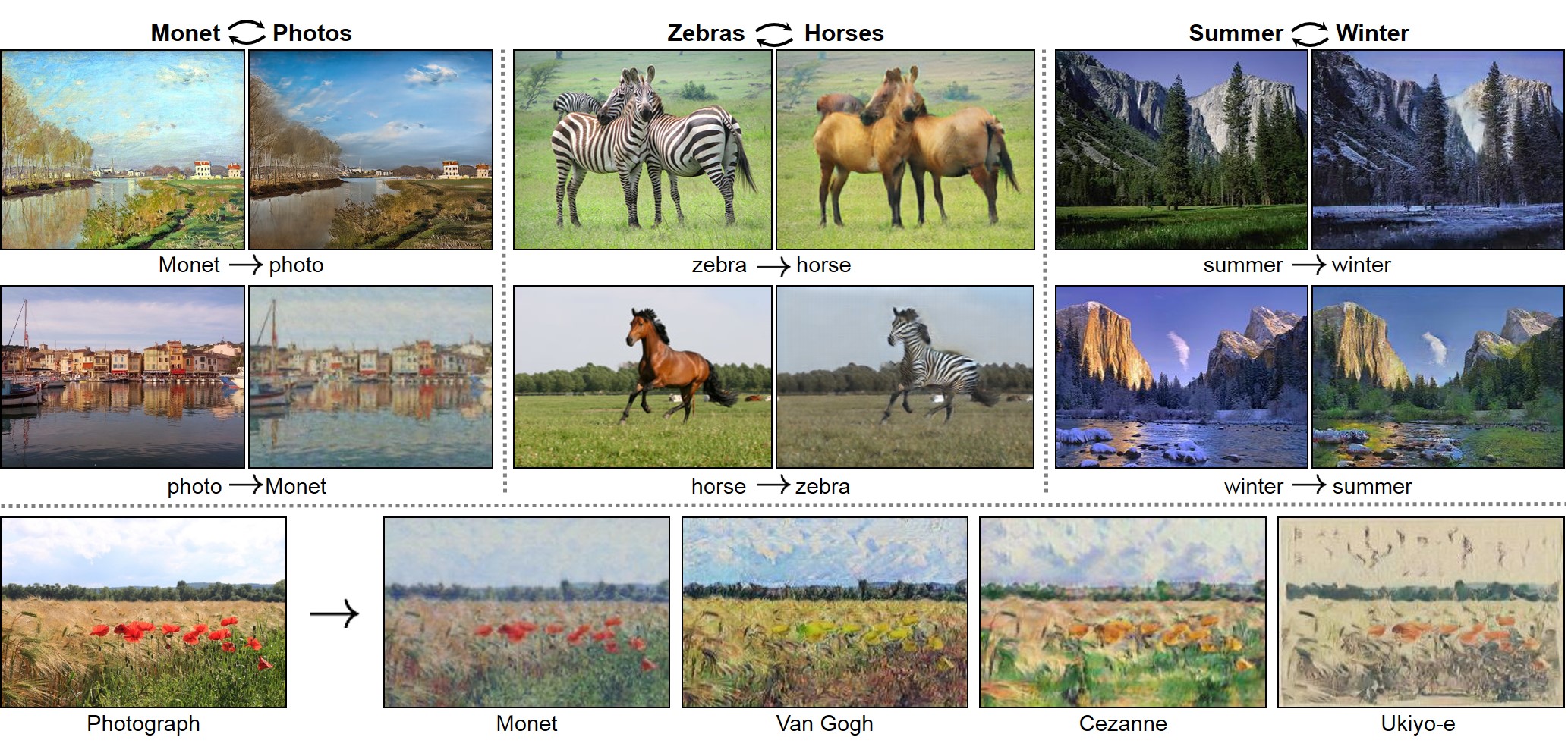
Domain adaptation is a subset of machine learning methods that act as translators, for example converting images taken in the daytime to look as if they were taken at night (see here for cool examples!). The main idea behind the translation is to hold fixed what the images have in common with each other and only change the context (day/night, summer/winter, etc.). What O’Briain and collaborators realized is that the synthetic gap can be viewed as a domain adaptation problem.
It might seem unthinkable to take a large number of labeled models and unlabeled observations and learn how to translate from one to the other. However, this is exactly what O’Briain and collaborators achieved with Cycle-StarNet, using domain adaptation methods to convert between the domain of models and domain of measurements of stellar spectra (the light we see from stars as a function of energy).
Key Insight: Force them to share
Cycle-StarNet is built around a more general class of models known as autoencoders. Autoencoders compress data from a high dimensional space (the data space) to a much lower dimensional representation (the latent space) before decompressing back into the data space. The goal of the latent space is to be large enough to capture all of the interesting variations in the inputs, but small enough to force variability unrelated to the physics of interest (often called “noise”) to be lost. The key idea in Cycle-StarNet is to use an autoencoder to compress both the models and observations, but force them to share the same latent space (see Figure 1). This latent space encodes the “most important” information about the differences between stellar spectra. The only distinction between the models and observations in Cycle-StarNet is that the observations also have a second latent space to capture effects not present in the models. These could be real variations in the observations due to the conditions of the instrument acquiring the data, but are not related to the star itself.
Let’s demonstrate how this solves the issue of labeling data-driven models. Suppose you have a function that can generate a synthetic spectrum from a set of physical parameters (Figure 1, top left). This synthetic spectrum is perfectly labeled, but may not match observed data perfectly. As shown in Figure 1, this spectrum is compressed to the shared latent space (vector Zsh). But, since that latent space is shared, we can decompress that information as if it were an observed spectrum (Figure 1, bottom right). Thus, we can obtain realistic spectra that look like observations, but are labeled from our physical models!

Figure 1: A schematic of Cycle-StarNet illustrating how it can translate between synthetic and observed (stellar) spectra through a shared latent space (Adapted from O’Briain et al., Figure 2).
The Struggle: Training
The difficulty is in learning the compression/decompression functions. Each of the boxes in Figure 1 is a neural network that we can view as a black box function learned by tuning thousands of parameters. The “Cycle” part of Cycle-StarNet comes from one of the most important parts of the training process. The whole network tries to perfectly reconstruct a spectrum that is translated from synthetic to observed back to synthetic space again, forming a closed “cycle.”
However, difficulties with this training procedure impose some of the most serious limitations on the method. These difficulties restrict the synthetic and observed domains to span a similar range of label space (e.g. range of stellar temperatures), meaning Cycle-StarNet struggles to generalize beyond the types of observed data it has seen during training. Further, the authors highlight that subtle biases can persist (when trying to use Cycle-StarNet to label observed spectra) despite the rigorous training procedure.
What does it buy you?
O’Briain and collaborators showed that using Cycle-StarNet to translate synthetic to observed spectra significantly reduced the synthetic gap, providing labeled synthetic spectra that looked much more like the observed spectra. In turn, this allowed them to better learn the labels of (and thus physical processes behind) unseen observed spectra. In addition, they provide a proof of concept on purely synthetic data showing that they could use the change in models as a function of the input parameters to learn about physics present in the observed data but missing from the models. However, a demonstration that Cycle-StarNet can be used to learn about new physics in real data remains to be seen.
The authors have provided all of the code on Github so you too can build a bridge between your models and data!
Figure used under CC BY 4.0.