
Title: Scaled Process Priors for Bayesian Nonparametric Estimation of the Unseen Genetic Variation
Authors and Year: Federico Camerlenghi, Stefano Favaro, Lorenzo Masoero, and Tamara Broderick, 2022
Journal: Journal of the American Statistical Association (https://doi.org/10.1080/01621459.2022.2115918)
The Unseen Features Problem
How many species in our ecosystem have not been discovered? How many words did William Shakespeare know but not include in his written works? The unseen species problem has applications in both sciences and humanities, and it has been studied since the 1940s. This classical problem was recently generalized to the unseen features problem. In genomic applications, a feature is a genetic variant compared to a reference genome, and the scientific goal is to estimate the number of new genetic variants to be observed if we were to collect more samples. Mathematically, if we have observed KN unique features in the N samples collected so far, how many new features can be discovered if we can collect M more samples? In this post, denoting the number of new features by UN(M), we review recent advances in Bayesian approaches to estimate U.
Scaled Process Priors
To estimate the number of unseen features is challenging because the total number of features is potentially infinite. Before observing any data, a Bayesian statistician uses a prior distribution to characterize their a priori beliefs about the features. Then, after seeing N samples, they can update these beliefs by combining the prior distribution and the existing samples into a posterior distribution. In particular, the posterior distribution of UN(M) predicts the number of features to be seen in M new samples. Completely random measures (CRMs) have been a popular class of prior distributions for this problem. Unfortunately, CRMs exhibit a questionable behavior: With CRMs, the prediction of U is determined by the sample size N. Consequently, CRMs do not incorporate feature information, such as the number of unique features KN and their frequencies, into the estimation. Moreover, the posterior distribution of U must be a Poisson distribution. Poisson distributions have been widely applied to study count data (such as the number of events to occur over some time) and they are specified by only one parameter. However, the challenging unseen-features problem requires a posterior distribution with more complex structures.
The authors (Camerlenghi et al.) demonstrate that scaled process (SP) priors can enrich the posterior estimation of U. Generalizing CRMs to SP priors, the posterior distribution of U becomes a mixture of Poisson distributions and depends on frequencies of existing features. This means the posterior distribution is more flexible and also includes more information from current samples. After improving flexibility of predictions, the authors further investigate Stable-Beta scaled process (SB-SP) priors to improve the tractability of calculations. With SB-SP priors, the posterior distribution of U is specified by the sample size N and the number of existing features KN. Moreover, this posterior distribution is a negative Binomial distribution, which is similar to the Poisson distribution but includes an additional parameter to allow for a higher variance. Table 1 summarizes the posterior inference of U using the three classes of priors.
Table 1- Summary of Priors for the Unseen Features Problem
| Prior family | Posterior family | Posterior depends on |
| Complete Random Measures | Poisson | N |
| Scaled Process | Mixture of Poisson distributions | N,KN and frequencies |
| Stable-Beta Scaled Process | Negative Binomial | N and KN |
How to Evaluate the Predictions?
Given N training samples, the quality of the new-sample predictions (see MathStatBites post https://mathstatbites.org/predicting-the-future-events/ for discussions on both within-sample and new-sample predictions) can be assessed by the percentage deviation from the truth in the held-out dataset of size M. The accuracy measure, denoted by 𝑣N(M), lies on [0,1] and equals 1 when the estimate is perfect. We want the estimation to be more than level 𝑣 ∈ (0,1) accurate with high probability. In other words, the probability P (𝑣N(M) > 𝑣) should be as large as possible.
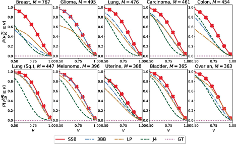
estimates are measured by percentage deviation from the truth, denoted 𝑣N(M), for 𝑁 = 10 training samples.
The authors test the empirical performance of the SB-SP priors using a cancer genomics dataset, Cancer Genome Atlas. For each of the 33 cancer types, they estimate the number of unseen genetic variants based on a training set with N = 10 samples. As reported in Figure 1, inference with the SB-SP priors (referred to as the SSB method) outperforms existing methods (stable-Beta process priors, linear programming, Jackknife, and Good-Toulmin estimators). To take a closer look, for breast cancer (top row first column), the SSB method is more than 𝑣 ≈ 60% accurate with probability almost 100%, when other methods achieve the same level of accuracy only around 60% of the time.
The Impact of Richer Predictive Structures
In the unseen features problem, we predict the number of features to be seen in the future M datapoints given the current N samples. In the experiments, the SB-SP priors perform well when the training size N = 10 is small relative to the extrapolation size M>300. But we benefit with more than just accuracy. The SP priors generalize the CRM priors and provide richer posterior structures for the unseen features. Knowing that CRM priors have been widely adopted by many applications, shall we also expect the SP priors to be more effective than CRMs in other contexts? Future research will tell us.