Review Prepared by: Moinak Bhaduri Mathematical Sciences, Bentley University, Massachusetts
Fine! I admit it! The title’s a bit click-baity. “Time” here need not be some immense galactic time. “Space” refers here not to the endless physical or literal space around you, but more to the types of certain events. But once you realize why the untangling was vital, how it is achieved in games such as soccer, and what forecasting benefits it can lead to, you’ll forgive me.
You see, for far too long, whenever scientists had to model (meaning describe and potentially, forecast) phenomena that had both a time and a value component, such as the timing of earthquakes and magnitude of those shocks, or times of gang violence and casualties because of those attacks, their default go-to were typical spatio-temporal processes such as the marked Hawkes (described below). While with that reliance no fault may be found in principle, the “right” usage of this model, where both the future times of occurrence and their related values may be predicted accurately, comes with strings attached. Heavy strings! Truly heavy strings! One issue that nearly strangles any forecasting analysis – killing it to the point of being unrealistic or impractical – is separability: the assumption that space flows independently of time. Much like insisting – and this is quite vital in this instance – that the magnitude of an earthquake has got nothing to do with when it occurs. But, in other examples, one may have a lot to do with the other. It is the loosening of these grips, the giving up of these assumptions, that Narayanan, Kosmidis, and Dellaportas in their article, “Flexible marked spatio-temporal point processes with applications to event sequences from association football” focus on, and, in the process, develop a brand of flexible alternatives to tackle contexts like predicting the times and the types of crucial events in a soccer game which may share odd similarities with earthquakes in certain ways and differ from them in others.
A neat kickoff to showcase current theoretical troublesThe authors demonstrate their methods with examples from football, or soccer, but do point out eventually that these may be deployed to other team sports such as hockey or rugby or even to contexts beyond sports. They lay out tables such as 1 and 2 below, made out of a Southampton-West Ham match played on 15th September 2013. You would notice (Table 1) each event has a time-stamp on it (just as an earthquake or a gang violence has a time-stamp on it) and there are many types of events (Table 2). While the time aspect is graspable, if we are seeking to find parallels, the type aspect could confuse. After all, if we’re tracking an earthquake sequence, all we witness are earthquakes – just jolts of different kinds. If we’re tracking gang violence, all we observe are fights and casualties. It could, therefore, be a leap of the imagination to realize how the magnitudes or amounts could be potential proxies for types: we can take major events, such as the scoring of a goal, to be the primary ones (like an earthquake or the first fight of a violence sequence) and minor events, like interceptions or clearances to be accompanying secondaries (like aftershocks or retaliations). If you want to nitpick technicalities: the mark space (i.e., the type of associated event categories) is discrete (i.e., either a goal, or a pass, or an interception, etc., and nothing “in between”), offering a probability mass function, instead of continuous (like the amount of rainfall which can be anything “in between” two numbers), triggering a density. This time-space co-operation is typically forced to conform to a fixed format:
$ \lambda^*(t, m)=\mu \delta_m+\sum_{t_j}\epsilon \beta \mathrm{e}^{-\beta\left(t-t_j\right)} \gamma_{m_j \rightarrow m^*}$ (1)
Here, the parameter $\mu>0$ is a constant background intensity and $\delta_m \in(0,1)$ is the background mark probability for mark $m$ with $\sum_{m=1}^M \delta_m=1$. The parameter $\epsilon \in(0,1)$ is the excitation factor, $\beta>0$ is the exponential decay rate, and $\gamma_{m, \rightarrow m} \in(0,1)$ is the probability the excitation from an event of mark $m_j$ triggers an event of mark $m$, with $\sum_{m=1}^M \gamma_{m_j \rightarrow m}=1$ for any $m_j \in{1, \ldots, M}$.
Table 1. Events and their attributes from the first 20 s of the game between Southampton and West Ham United on 15 September 2013
Second Minute Team_id Player_id Type $x$ $y$ Outcome End_ $x$ End_ $y$ 1 0 14 29,544 Pass 50.1 48.8 Successful 51.1 48.2 2 0 14 21,683 Pass 51.1 48.2 Successful 39.2 47.8 4 0 14 71,714 Pass 39.2 47.8 Successful 29.5 77.6 6 0 14 118,244 Pass 30.8 79.6 Unsuccessful 33.5 79.7 12 0 20 12,533 BallRecovery 34.9 89.9 13 0 20 12,533 Pass 35.9 88.3 Successful 37.3 76.1 15 0 20 8,247 Pass 34.9 77.0 Unsuccessful 44.9 85.9 16 0 14 71,714 Interception 53.2 16.7 18 0 14 69,375 Pass 43.1 23.1 Unsuccessful 70.9 9.7 Note. For each event, we have records of the event time-stamp, team and player ids, event type, ( $x, y$ ) co-ordinates of its location in the playing field, and if the event type is a Pass, the event outcome (successful/unsuccessful) and the end ( $x, y$ ) co-ordinates.
Table 2. Frequencies of the 22 distinct types of touch-ball events in the data
Narayanan, Kosmidis, & Dellaportas 2023
Event type Frequency Event type Frequency Pass 376,924 SavedShot 4,971 BallRecovery 36,908 Save 4,910 Clearance 25,462 CornerAwarded 4,100 Tackle 14,581 MissedShots 4,076 TakeOn 13,607 OffsidePass 1,582 BallTouch 13,517 Claim 1,181 Aerial 12,871 Goal 1,052 Interception 10,422 Punch 380 Dispossessed 8,897 ShotOnPost 187 Foul 8,238 Smother 122 KeeperPickup 5,208 CrossNotClaimed 81
This, technically, is the joint intensity of marks and times and tells us – once we set a time window on it, and a mark type – how likely it is to find that type of an event over that time window: the higher the intensity, the more likely. Consider a period of play between the 15- and 20-minute marks. If, over this period, the background intensity in equation (1) is high, that would indicate many interesting events have happened but won’t precisely point out what kinds of events they were. To know this, we need to look into the mj→mprobability factors (m’s represent the types of events). If, over this period, int→dis is 0.7 and s.pass→s.pass is 0.2, then many of those interesting events will be where an interception led to dispossession, and fewer will be where a successful pass led to another successful pass. Because equation (1) can shed light this way on both the times and the types of events, it is termed the “joint” intensity. It is the successive adding up of times in the above equation that causes certain problems. Chief among which is the unavoidable clustering of times. Note each time an event happens, intensity (1) moves up a bit, claiming other events would be more probable in the future. This could prove questionable in a soccer setting. We may expect a dispossession to follow close on the heels of an interception, but it is unrealistic to expect two interceptions to be close in time (the authors, in fact, document in Figure 4 of their work how this is truly unrealistic). So, we expect the types of events, the marks, to cluster, but not quite the event times. If one insists that a joint intensity such as (1) should describe the full evolution of the spatio-temporal process, there is no way to incorporate this expectation. This is precisely where the authors innovate.
The crucial interception
Many of us tend to dismiss old observations. We disregard their insights and take what they point to as irrelevant relics. Thankfully, here, the authors stayed curious. They dusted the cobwebs off a 1975 result shown by D.R. Cox that factorized the likelihood (in case you need a refresher on likelihoods: https://www.sciencedirect.com/topics/medicine-and-dentistry/maximum-likelihood-method) of a marked point process over a time window (0,T] as
$\mathcal{L}\left(\mathcal{F}{t_n} \mid \zeta, \theta\right)=\prod{i=1}^n\left{g\left(t_i \mid \mathcal{F}{t{-1-1}} ; \zeta\right) f\left(m_i \mid t_i, \mathcal{F}{t{i-1}} ; \theta\right)\right}\left{1-G\left(T \mid \mathcal{F}_{t_n} ; \zeta\right)\right}$ (2)
Those familiar with standard time-truncation ideas may notice the smell of survival analysis (in case you need an explainer: https://sphweb.bumc.bu.edu/otlt/mph-modules/bs/bs704_survival/BS704_Survival_print.html) in the last factor where the fact that you have not witnessed an event over the last window also contributed a piece to the likelihood. The authors encourage us to give up our attachment to (1). Instead, they show how to derive the specification of the marks from an equivalent representation that will enable us to ensure the marks excite themselves: that is, an interception, for instance, triggers a dispossession. And then – and this is vital – once that is done, how to specify whatever probability distribution we need for the times that best serves our soccer ball contacts. These time distributions need not be made in a way that demands the time values are clustered. Which is what we wanted: the types clustered, but not the times. Time is liberated, so to speak, from space. The strategy is similar to factorizing a number such as 96 (the joint intensity) into pieces (the conditionals) that best suit our purpose. They could be 48 and 2. Or – if we want the first to be smaller – 12 and 8.
In addition to this general or main innovation, the authors have looked at other complications. The conversion probabilities in the mark space we find in (2) that is, the chances an interception will lead to a dispossession, or a corner will lead to a goal, will realistically depend on the location of the ground where the ball is in play. For instance, the home team will have a stronger chance than the away of an interception leading to dispossession, when the ball is in their half. We are shown a way to polish these probabilities taking these relevant details into account. Just as we are shown how to estimate parameters involved in (2) using readily available packages in the software STAN.
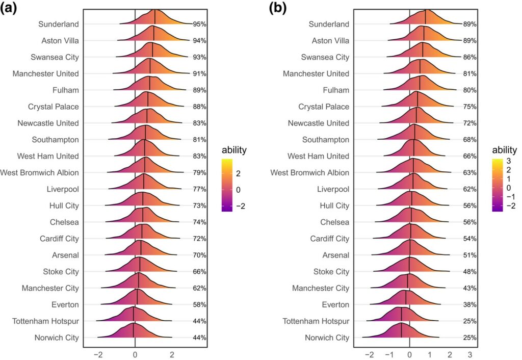
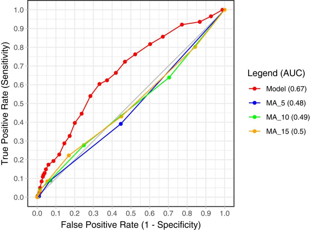
The disentanglement was not just a theoretical nicety. Through the new framework and the Bayesian posteriors (i.e., updated beliefs on event times and types) it uses, we can work out a given team’s ability of converting a ball-snatch to a successful pass while playing at home relative to playing away (the first panel in Figure 1, shown below) or converting a successful pass to another (the second panel). These were local or granular details. Global or game-level inferences can be furnished as well. In case you’re curious about prediction – whether a shot on goal will happen in a given 30-second window – the fresh model demonstrably (the Receiver Operating Characteristic curve, or ROC, in Figure 2, shown below) outperforms its established competitors, sounding neither too many false positives nor false negatives.
Some post-match punditry
Well, I meant some “final thoughts” on the research article… I just can’t seem to shake off the soccer hangover. Sorry! The point is: marked or Hawkes, that is, self-exciting point processes (that is, occurrence patterns of events that make other events more likely in the immediate future) have already been used in a variety of contexts in a fixed format. Perhaps while we examine works such as the current, we can salvage and still boast of a remnant of a heritage the tide of repetition has

swept away. While the work is stunning, we, as critics, relish the pointing out of the inevitable collision between the achievement and its potential or promise. With similar data readily available on the internet, soccer enthusiasts, whatever their technical backgrounds, may jump in. There’s plenty to innovate for everyone.
Events in the field are frequently affected by those outside: the decisions from the managers, crowd involvement, etc. More sophisticated intensities (that is, other ways of reporting equation 1, other ways of showing how the timestamps and the types of events mesh and clash once we are conscious of these external factors; for instance, as a manager makes a replacement right after a goal was conceded) would take these into account.

Is this the only format of disentanglement? Of setting time free from space? Hardly! Newer versions of decoupling may come along before long. Until then, this work would remain popular chiefly because the authors were able to express in a catchy, implementable, and therefore, memorable form the native generalizability of a self-exciting framework that have stayed steadfastly irreplaceable.
References
Santhosh Narayanan, Ioannis Kosmidis, Petros Dellaportas, Flexible marked spatio-temporal point processes with applications to event sequences from association football, Journal of the Royal Statistical Society Series C: Applied Statistics, Volume 72, Issue 5, November 2023, Pages 1095–1126, https://doi.org/10.1093/jrsssc/qlad085
D. R. COX, Partial likelihood, Biometrika, Volume 62, Issue 2, August 1975, Pages 269–276, https://doi.org/10.1093/biomet/62.2.269

