Title: Nested sampling with any prior you like
Authors and Year: Justin Alsing and Will Handley (2021)
Journal: Monthly Notices of the Royal Astronomical Society: Letters
Nested Sampling
In order to validate our understanding of the world around us, we want to compare theoretical models to data we have actually observed. Often, these models are functions of parameters, and we want to know the values of those parameters such that the models most closely represent the world. For example, we may believe the concentration of one molecule in a chemical reaction should decrease exponentially with time. However, we also want to know the rate constant, the parameter in the model that multiplies time in the exponential, such that the model exponential curve actually resembles a specific reaction that we observe. This is the problem of parameter inference, for which we often turn to Bayesian methods, especially when working with complex models and/or many parameters.
In this Bayesian parameter inference framework, we compute the probability of a combination of parameters given the data, known as the “posterior,” as a product of two terms. The first is the “prior,” which is the probability we ascribe a combination of parameters before an observation. The second is the “likelihood,” which is the probability the data would have been observed given that the proposed parameters were the true ones. Then, Monte Carlo methods estimate the posterior by evaluating the likelihood and prior at a large number of points in parameter space. Different families of Monte Carlo methods are differentiated by how these sample parameter points are chosen.
Nested sampling is a popular Monte Carlo method for Bayesian parameter inference because it can handle complicated shapes for the probability distributions. However, it does this by starting with draws from the prior distribution. Therefore, most implementations require a simple (often analytic) function that converts the prior distribution to the unit cube (values between 0 and 1), which can be easily sampled.
Parametrizing the Prior Map
Alsing and Handley point out that parametric maps, functions that depend on a large number of additional free tuning parameters, could be used to convert between the prior and unit cube instead of requiring a function that is a simple equation, thereby enabling a much broader range of prior distributions for use with nested sampling. In a simple case, these parametric maps could be compositions of multiple invertible functions (such as sinh and arcsinh) with tunable additive or multiplicative constants (“m” and “b” below, respectively).
f(x) = sinh(mx+b )
However, more modern approaches generally rely on normalizing flows, which use neural networks to parametrize the map and can express a wider range of possible functions by tuning a large number of constants. While theoretical guarantees on the expressiveness of normalizing flows to represent many types of distributions are comforting, the most convincing argument is that authors demonstrated this prior specification formalism works in practice.
How to combine two experiments?
One of the most exciting applications of these flexible prior maps is the ability to use the posterior from one inference as the prior for a second inference with new information. This sort of sequential combination of experiments is generally inhibited by the lack of an exact functional form of the posterior from the first experiment. Alsing and Handley demonstrate this sequential combination of experiments for the problem of inferring parameters of models of the universe, known as cosmological parameters. They consider two data sets: measurements of (1) the cosmic microwave background (CMB), which is light from the early universe, and (2) the baryon acoustic oscillation (BAO) as measured by galaxy clustering. Both probe fluctuations in the universe at intergalactic distance scales.
Figure 1 is a series of plots showing probability distributions over two of the cosmological parameters being inferred, H0 (the Hubble constant) and Ωk (spatial curvature parameter). The top plot shows the original theoretical prior distribution for what combination of parameters is possible. In the middle panel of the second row, the posterior using nested sampling with both data sets is shown. For every step in the sampling, this requires computing the likelihood for both the CMB and BAO data. Further, because the prior distribution is large, the inference requires many samples to arrive at the posterior.
The left and right columns of the second row show the posteriors obtained using only the CMB or BAO data, respectively. The third row is what is made possible by the flexible prior specification, where the posterior from one experiment is used as the prior for the next inference step with the other experiment. The key result of the paper is the comparison in the middle of the bottom row. The fact that shape of the posterior for all three colors almost exactly overlaps shows that the final posterior combining both the CMB and BAO data is practically identical between all three routes shown (joint CMB BAO likelihood inference, CMB as prior for BAO inference, or BAO as prior for CMB inference).
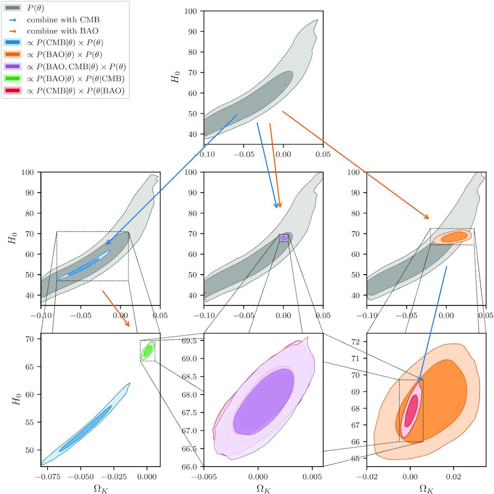
Figure 1. A comparison of cosmological parameter inference combining two different datasets (CMB and BAO) simultaneously and sequentially in either order. The similarity of the final posterior for all three inference methods validates the sequential inference approach enabled by normalizing flows discussed in the paper (Adapted from Alsing and Handley, Figure 1).
One of the major benefits of combining the information from experiments sequentially is that the size of the prior space for the subsequent inferences is reduced by the first experimental constraints. This reduces the number of samples required for the inference, which can significantly reduce runtime when the likelihood is expensive to compute.
The Flexible Prior Function Future
Readers interested in the implementation used by Alsing and Handley can head over to Zenodo to access their modified version of the code CosmoChord. Excitingly, they also plan to release a library of cosmological priors based on different experiments as a service to the community. This library would streamline analyses of and comparisons to new experiments seeking to constrain cosmological parameters. However, the devil is in the likelihood, and often in the data uncertainties themselves entering the likelihood. So, while simplifying prior specification certainly aids in the analysis, it doesn’t make the interpretation of the inferred posterior any easier.
Figure used with Permission from MNRAS