Whatever your exact interests in data, frequently, inseparable from model-building, stand other related responsibilities. Sample two crucial ones:
a. the checking of how well your model did: the less frequently you make big, bad decisions – like predicting someone’s salary to be $95,000, an estimate far adrift from the real, say, $70,000 in case it’s a regression problem, or saying a customer will buy a product when, in fact, she won’t, under a classification environment – the happier you are. These accuracies are unsurprisingly, often used to guide the model-building process.
b. the explaining of how you arrived at a prediction: this involves unpacking or interpreting the $95,000. The person, due to his experience, makes $10,000 more than the average, due to his education, makes $20,000 more, but due to his state of residence, makes $5000 less than the average, etc. These ups and downs contribute to a net final value.
For standard linear or logistic regression, these tasks are quite routine. For more recent machine learning offerings, such as random forests or boosted trees, interpretability issues are being tackled in innovative ways. Partial dependence, interaction plots and refinements such as Shapely diagrams (https://christophm.github.io/interpretable-ml-book/shap.html) are emerging at an assuring pace.
In unsupervised contexts, however, that is in situations where there is no right answer – the $70,000, or the “not buying”, tasks (a) and (b) may pose quite some challenge, in the absence of benchmarks against which our estimates may be compared. Clustering is such a context. Based on features, i.e., details of people or objects, the chief aim is to put them in groups so that members in a group are similar in some sense and those in different groups are dissimilar. A way of stereotyping, you could argue. There is no notion of the right group assignment. Nor is there a way to explain away why – that is, due to which feature, which piece of detail, an individual got dragged into a given group. This doubtless erodes our trust in them and hinders troubleshooting. Clustering methods you may have seen, such as the k-means algorithm, routinely tolerate these imprecisions. It is amidst this chaos that practitioners crave some much needed order. The situation, however, has spawned a breed of incurable optimists. Meet three of them: Nicolas Dugue, Jean-Charles Lamirel, and Yue Chen. Teaming up, determined to make matters interpretable, they’ve written “Evaluating clustering quality using features’ salience: a promising approach” to install a firmer system. Their instrument? A fraction called the F-measure. Easy to grasp, its connection with a feature’s relevance seems not only illuminating but inevitable.
The salience of salience
Let’s be candid. The key goal here is not to produce newer ways of doing clustering – although the tools shown here may trigger newer ways – rather, it is checking how neat the groups are – task (a) above – and explaining why the groups are that way – task (b) above, once the clustering is done through some method, good or bad. An algorithm serving a fashion retailer – bent of profiling customers, may, as a pilot study,
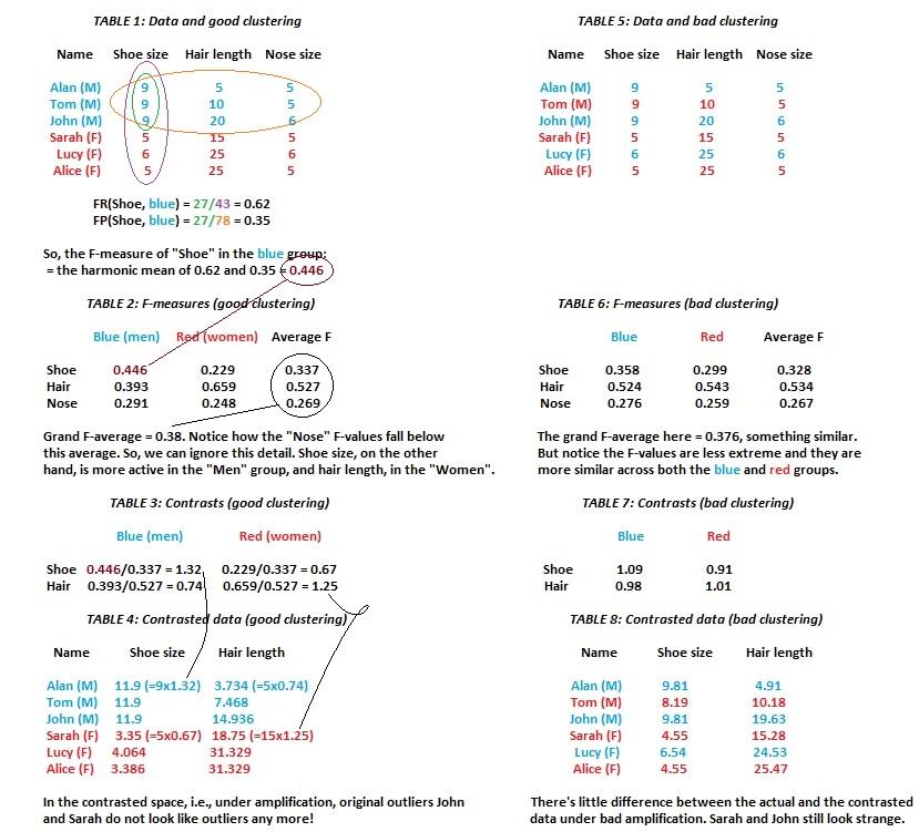
want to group six individuals, shown in Table 1, on the basis of their shoe size, hair length, and nose size. Some observations are immediate and intuitive. The men, in comparison to the women, have in general, larger shoe sizes and smaller hair. A good clustering method may detect there are these two main types of individuals (which we, but not the method, know as “men” and “women”) while a weaker method may miss this point either totally, or may take some women to be men and some men to be women. The authors put forth a way both to identify the first method as the better of the two – task (a) – and to reveal which feature out of the three (shoe size, hair length, and nose size) gave rise to the two groups – task (b). Here is the critical insight:
A feature’s recall (FR) shows how regularly that variable takes a certain type (big or small) of value in a given group (please check Table 1). The more regularly it picks a side, the more extreme its recall value, i.e., the more able it is to separate one group from the other.
A feature’s predominance (FP), on the other hand, shows, in relative terms, how big of a share that property has within a given group. The bigger the share, the more that group depends on that property to describe itself.
The authors note that any feature worth its salt should play a major role in these two jobs – helping separate one group from the other, and ensuring a group depends on it heavily. They take, therefore, the average (the harmonic mean, to be precise) of these two fractions to describe the grand relevance – the salience – of a feature, within this clustering business. Formally, this mean is termed the F-measure. Unsurprisingly, under the good clustering, you would notice, shoe sizes’ grand salience is high for the men and low for the women while hair lengths’ grand salience is the other way around – something which confirms our initial intuition. Observe, simultaneously, that under the bad clustering, that is, when the men-women separation was not as solid, the F-measures for any feature didn’t quite pick a clear side. None of the features, therefore, is quite so responsible – so to speak – for this bad grouping, making it a lot less interpretable.
Is this the only way to tell a neat grouping from a messy one? Exploiting interpretations? Not at all. Euclidean-type metrics do that job through calculating the distance between the cluster centers (levying equal importance on all features, even silly ones, like our “nose size”). They, sadly, are not so easily explainable – i.e., they won’t say which features are predominant in which group and fail under high dimensionality – i.e., when we have a lot of details to worry about, not just three.
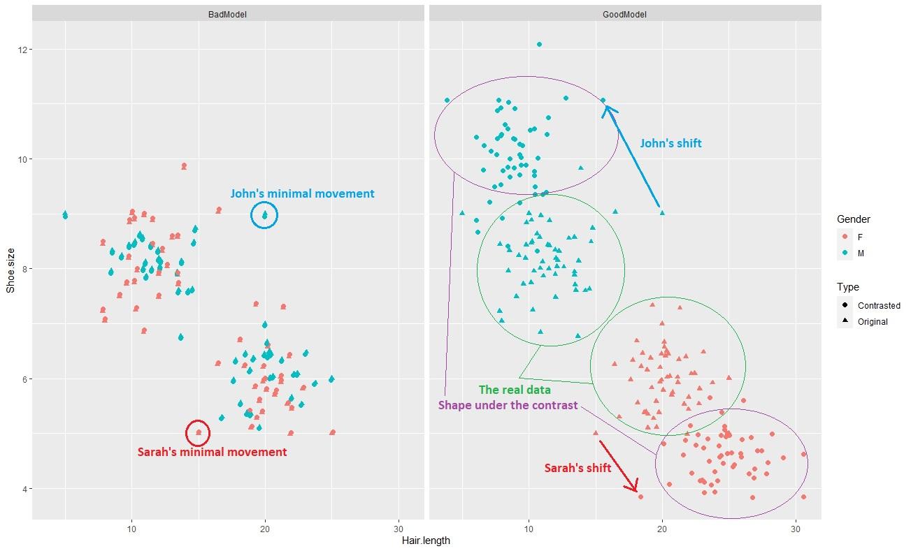
Fig 1. Contrasts at work on a larger data set. Good – i.e., explainable clusters generate good contrasts which impart a pulling force, neatly unentangling any initial overlap that may have remained due to weird outliers.
And oh, we can sort out nagging troublemakers too!
There are many wills to which you can bend your F-measure. One could be feature-screening – weeding out details irrelevant to the clustering, another could be fixing outliers. The authors recommend looking at the overall average F-measure (average calculated across all feature-group combinations) to set a standard and removing the ones who do not reach this standard. This deleted detail, for us, again, not unexpectedly, is “nose size” (Tables 2 and 3).
Once we identify a good set of features, i.e., those details that really lend some meaningful aid in locating one group or the other (evidenced through their high F-values) we can construct “contrasts” to remedy strange observations. Take John, for instance. His hair is as long as a typical woman’s. Or Sarah, for that matter, whose hair is as short as a typical man’s. Unusual observations such as these trick the standard the Euclidean distances, making the two groups seem closer than they are (panel two, figure 1). Contrasts rectify these anomalies. Through some transformations, they make John’s hair as short as the typical man’s and Sarah’s as long as the typical woman’s. In a case where our six individuals are part of a bigger crowd (Figure 1), such alterations – which geometrically represent a shift – make the groupings a lot more vivid, pulling one cluster farther away from the other. Computationally these contrasts are not taxing, either. We simply need to calculate the above or below-average importance (Tables 3 and 4) each relevant feature exerts within each group and multiply our original data values with these fractions to construct these contrasted values.
Dugue, Lamirel, and Chen have described these notions using keywords within French and English texts, but the idea of a feature’s salience (quantified through its F-measure) remains the chief intellectual mainstay. With regards to the choice of a clustering tool, one doesn’t find any sense of advocacy. Practitioners may choose clustering techniques according to their temperament or instinct. The authors do not enforce a specific method – the k-means, or some such. The special splendor of their work is in supplying reasons behind the grouping – these add-ons – shouldering duties (a) and (b), while allowing that freedom. While interpretability concerns have been rightly attracting attention in a supervised setting, it is the tragic temper of our time that its opposite circumstance – the unsupervised scene had endured steady neglect. Modest in its construction but vaulting in its ambition, the F-measure transmits some urgency in this complementary space, no matter the obstacles – high dimensions, outliers. A promising vehicle totters into motion! Take heed!
References:
The main article: Dugué, N., Lamirel, JC. & Chen, Y. Evaluating clustering quality using features salience: a promising approach. Neural Comput & Applic 33, 12939–12956 (2021). https://doi.org/10.1007/s00521-021-05942-7
Online: https://christophm.github.io/interpretable-ml-book/shap.html