
Title: Crime in Philadelphia: Bayesian Clustering and Particle Optimization
Author(s) and Year: Cecilia Balocchi, Sameer K. Deshpande, Edward I. George & Shane T. Jensen, 2023
Journal: Journal of the American Statistical Association, Applications and Case Studies: https://doi.org/10.1080/01621459.2022.2156348 (open access)
“Violent crime fell 3 percent in Philadelphia in 2010”1 – this title from the Philadelphia Inquirer depicts Philadelphia’s reported decline in crime in the late 2000s and 2010s. However, is this claim exactly what it appears to be? In their paper, “Crime in Philadelphia: Bayesian Clustering and Particle Optimization,” Balocchi, Deshpande, George, and Jensen use Bayesian hierarchical modeling and clustering to identify more nuanced patterns in temporal trends and baseline levels of crime in Philadelphia.
What is Bayesian Hierarchical Modeling?
To understand Bayesian hierarchical modeling, it helps to go over Bayesian models. Bayesian models have three main components: the prior, the likelihood, and the posterior.
Let’s work in the context of our example. Let’s say that we have data on crime densities (defined as the number of violent crimes divided by land area) for all neighborhoods in Philadelphia, and we are interested in estimating the mean crime density level for each neighborhood.
The prior and the likelihood together can be thought of as a two-step data generating process. For a given neighborhood:
Step 1: We will first generate a value for the mean crime density level from a probability distribution. We call this distribution the prior. The key idea behind the prior is that it is chosen to incorporate the researcher’s current beliefs about the mean crime density.
Step 2: We will now utilize the mean crime density from Step 1 to generate our observed crime density level, i.e. our data. The probability distribution we generate the data from is called the likelihood.
In short, the prior and likelihood together can be thought of as our proposed model.
In estimation, the key idea is that we want to use our observed crime density data to update our beliefs. This update is computed as the distribution of mean crime density given the observed data — we call this the posterior.
Bayesian hierarchical modeling extends these ideas and allows you to add more sub-models to the hierarchy to capture more complex relationships. Like regular Bayesian statistics, you will update your beliefs via the posterior.
One attractive feature of Bayesian hierarchical modeling is that it allows for the “sharing of information”. In this context, the authors believed that adjacent neighborhoods were likely to have similar crime densities. Therefore, when looking at a given neighborhood, we can gain more information by also looking at adjacent neighborhoods. Bayesian hierarchical modeling can model this by using a prior that encourages spatially close neighborhoods to be somewhat similar.
A Twist on Bayesian Hierarchical Modeling
However, in this setting, this approach does have one notable hiccup – there exist sharp boundaries where this type of assumption does not hold. For example, two neighborhoods may be separated by a river, and thus are not as similar as one would expect. Alternatively, two adjacent neighborhoods may differ drastically in the average socioeconomic status.
To account for this, the authors proposed a variant of this methodology that instead finds clusters of neighborhoods that are similar, and then uses desired priors within each cluster to estimate the quantities of interest. This process was used to estimate both baseline crime density and the trend in crime density over the period 2006-2017. To find these clusters, the authors developed an optimization technique that aims to find the cluster arrangement with the highest posterior probability. (I will not go through the details, but in short, this is done iteratively by testing a subset of “moves” to change the cluster assignment and checking for improvements. If you’re interested in learning more, check out the paper!)
The Results
Below is a visualization of the results for the cluster assignment of highest probability.
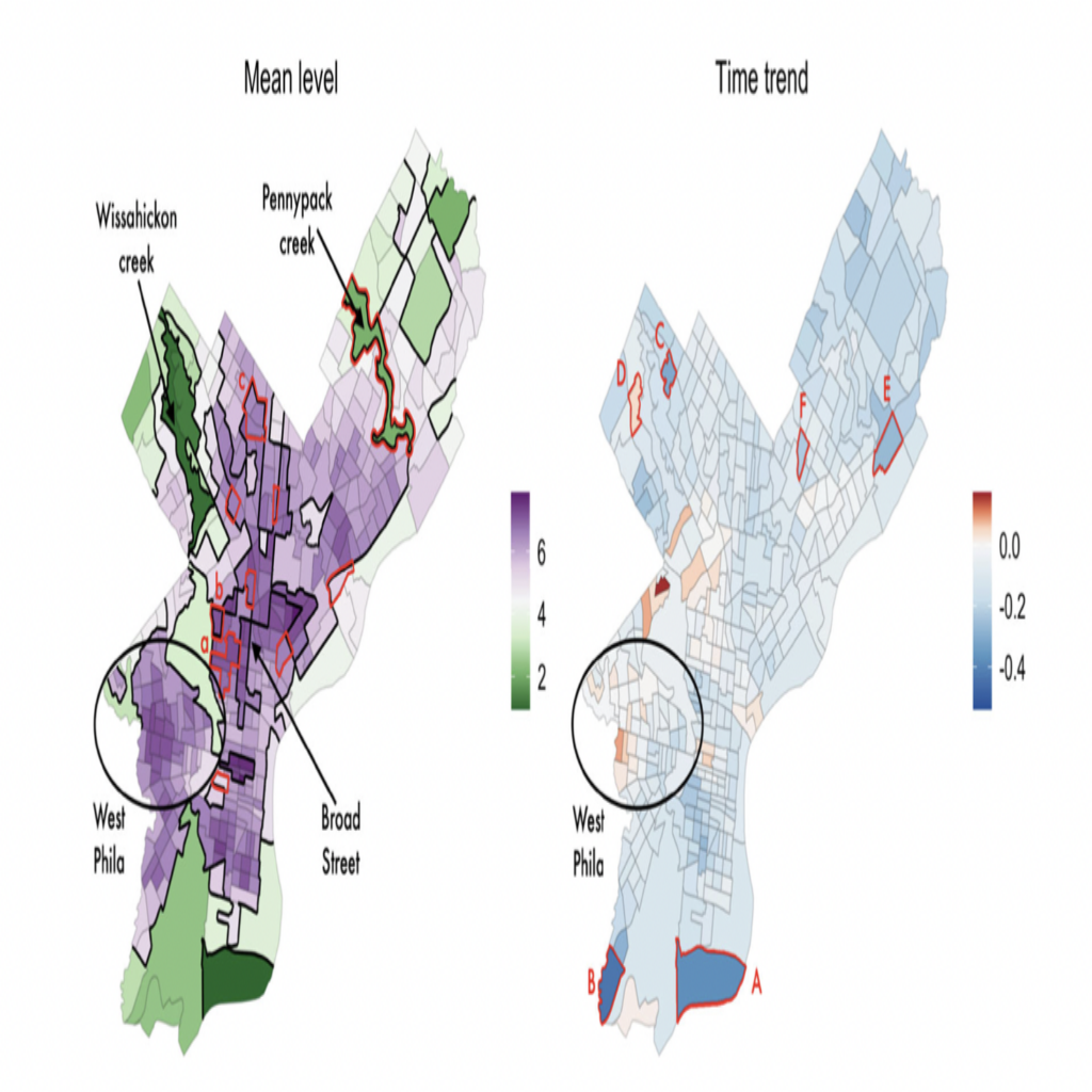
Fig 1. These are visualizations of the results corresponding to the cluster assignment of highest probability (superimposed onto a map of Philadelphia). The image on the left is a spatial visualization of the cluster and estimates for the baseline level of crime density. The image on the right is a spatial visualization of the clusters and estimates for the trend of crime density over time. Dark black lines are borders for the clusters. Red lines outline neighborhoods that were given different cluster assignments in other arrangements that had lower posterior probabilities. From Figure 5 in the paper. Figure used under CC BY-NC 3.0.
Analyzing the results unveils some features of the city that potentially influence the varying crime density. The first features are parks and rivers. In the picture on the left, there are two clusters, labeled Wissahickon creek and Pennypack creek, which have lower crime rates compared to adjacent neighborhoods. These two clusters correspond to parks next to rivers. Another feature is Broad Street. Broad Street acts as a boundary for many clusters, indicating that crime densities may change when crossing this road. An additional feature is the University of Pennsylvania (UPenn). UPenn is in the east section of the West Phila cluster which covers the West Philadelphia and University City neighborhoods. From the picture on the right, we see the east side of the section saw a decrease in crime while the west side saw an increase. This pattern is likely related to UPenn’s West Philadelphia Initiatives program, which aimed to improve the area surrounding the university.
Overall, the authors found that the claimed decrease in crime in Philadelphia was not uniformly present across the city. Their methodology does have some areas of improvement (which are also potential areas for future research!) One example is incorporating neighborhood data in the model. However, the method shows promising results which can lead to a better understanding of crime patterns. Hopefully, these findings can impact resource allocation and/or policymaking that will improve the quality of life for all of Philadelphia’s residents.
[1] Graham, T. (2010, December 30) Violent crime fell 3 percent in Philadelphia in 2010. Philadelphia Inquirer. https://www.inquirer.com/philly/news/homepage/20101230_Violent_crime_fell_3_percent_in_Philadelphia_in_2010.html