Article: Gaussian graphical models with applications to omics analyses
Authors and Year: Katherine H. Shutta, Roberta De Vito, Denise M. Scholtens, Raji Balasubramanian 2022
Journal: Statistics in Medicine
Review Prepared by: Sanou Edmond, Postdoc in Biostatistics
Nuclear Safety and Radiation Protection Authority (ASNR)
As scientists collect more detailed biological data, they use networks to understand how molecules in the body interact and how these interactions relate to disease. This type of data, known as omics, includes information about genes (genomics), proteins (proteomics), and other molecules. These networks can help find genes linked to illness and even suggest possible treatment options. Statisticians help by using tools that highlight which molecules are directly connected. In their tutorial “Gaussian Graphical Models with Applications to Omics Analyses,” Shutta et al. recommend using a method called Gaussian Graphical Models (GGMs) to study these connections. GGMs help draw simple, clear maps of how molecules relate to each other. The authors show how to apply this method using real ovarian cancer data and share example code to help other researchers use the technique more easily in their own work.
Gaussian Graphical Models
Gaussian Graphical Models are tools used to map how variables, like genes or proteins, are directly connected, especially in complex biological systems. Each variable is shown as a node in a network, and connections between nodes represent direct relationships that remain even after accounting for all other variables in the system.
A key concept is conditional independence, which helps us tell apart direct and indirect associations:
- Two variables are independent if they’re unrelated, regardless of what else is happening.
- Two variables are conditionally independent if they appear related at first but that link disappears when we account for (or “condition on”) a third variable or set of variables.
To help visualize this idea, consider the following figure:
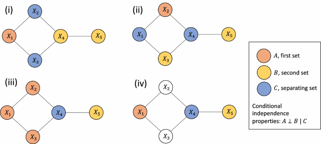
This diagram shows four different network setups where sets of variables (colored nodes) are analyzed for conditional independence. Here’s what each panel shows:
- (i): X1 and X4 are conditionally independent given X2, X3 . There is no path from X1 to X4 that doesn’t go through X2 or X3.
- (ii): X2 and X5 are conditionally independent given X4 . Again, X4 “blocks” all paths.
- (iii): X1 and X5 are conditionally independent given X4 , showing a different configuration but the same principle.
- (iv): X1 and X5 are conditionally independent given X4 , and here, only the relevant conditioning node is colored to highlight the path-blocking concept.
In each case, the blue nodes (C) act as a “separating set” between the orange (A) and yellow (B) nodes, demonstrating the key idea: If all paths from A to B pass through C, then A and B are conditionally independent given C.
This visualization makes it easier to grasp how GGMs uncover direct relationships by distinguishing them from indirect ones, important for interpreting high-dimensional biological data.
Estimation of a Gaussian Graphical Model
This section talks about how researchers figure out which variables in a dataset are directly related to each other, using the Gaussian Graphical Models. The idea is to look not just at whether variables are associated, but whether they are directly connected after accounting for all the other variables. To do this, we start with something called a covariance matrix, which is a big table that shows how much each pair of variables tends to vary together. For example, if two variables both increase or decrease together a lot, their covariance will be high.
To get more specific information about direct connections between variables, researchers often use a version of this matrix called the precision matrix. This matrix tells us which variables are directly linked, in the sense that their relationship can’t be explained away by other variables. The precision matrix can be obtained by inverting the covariance matrix, but this only works well when there are more samples than variables. If there are more variables than data points, which often happens, the matrix can’t be inverted, and the method breaks down.
To deal with that, researchers use something called regularization. This just means adding a rule that pushes some of the connections in the precision matrix toward zero, which helps create a simpler, easier-to-interpret network. Even when we can invert the matrix, regularization is useful because it helps focus on the strongest and most meaningful connections.
One early regularization method came from researchers Meinshausen and Bühlmann, who looked at one variable at a time and figured out which other variables helped predict it, using linear regression. If a variable helped predict another, it was considered directly connected in the graph. This approach helped identify the network structure, though it didn’t give exact values for the strength of each connection.
Later, more precise methods were developed, most notably the Graphical Lasso, introduced in 2008. This method fine-tunes the balance between capturing the data and keeping the graph simple by adding a penalty for complexity. It became the standard way to estimate GGMs, especially in situations with many variables. Researchers later found a clever way to break this big problem into smaller, faster parts, making it possible to analyze massive datasets quickly.
Application on ovarian cancer data
The paper used gene expression data from a study on ovarian cancer published by The Cancer Genome Atlas, accessed via the curatedOvarianData R package. An R package is a collection of functions, data, and documentation bundled together to make it easy to perform specific tasks in R, which is a popular programming language used for statistics and data analysis.
This dataset consists of a 13,104 × 578 matrix:
- Rows represent genes,
- Columns represent individual patients,
- Cells contain preprocessed gene expression levels.
| TCGA.20.0987 | TCGA.23.1031 | TCGA.24.0979 | TCGA.23.1117 | |
| A1CF | 2.923522 | 3.052169 | 2.846371 | 3.002209 |
| A2M | 10.353008 | 11.635772 | 7.954542 | 9.9715 |
| A4GNT | 3.321405 | 3.666463 | 3.258038 | 3.596212 |
| AAAS | 4.60801 | 5.142133 | 5.025422 | 5.139928 |
| AACS | 7.279213 | 7.048869 | 7.750161 | 6.206031 |
Table of Gene Expression Data: Expression levels of the first four genes across five participants from the ovarian cancer dataset.
The table above shows a small snapshot of this data. Each row is a gene (like A1CF, A2M), and each column is a patient (e.g., TCGA.20.0987). The numbers indicate how strongly a gene is expressed, or “turned on”, in a given patient. These values help researchers identify patterns that distinguish different types of tumors or suggest how the disease might be progressing.
Before using this data to build a network with a Gaussian Graphical Model (GGM), it’s important to standardize the gene expression values. In simple terms, standardization is like resetting the scale for each gene so that they can be fairly compared. Without it, genes that naturally have higher values might dominate the analysis, not because they’re more important, but simply because they use a different scale. For example, imagine measuring two things: one in meters and one in millimeters. Without adjusting the scale, the numbers in millimeters will look much bigger, even though they represent the same physical quantity. Standardization fixes this by adjusting all variables to have a similar scale, typically by centering them around zero and making sure they have similar spreads. This step is especially important in biological data, where the actual units may not carry direct meaning. In fields like metabolomics, for instance, values often represent relative levels of molecules, not exact amounts. So standardizing helps focus the analysis on patterns of variation between genes, rather than being misled by arbitrary differences in measurement scale.
To estimate a Gaussian Graphical Model, the glasso function from the glasso R package is applied. A regularization parameter, called rho must be specified. This parameter controls how many connections appear in the resulting network by shrinking weaker relationships toward zero. Smaller values of rho produce more connected networks, while larger values lead to networks with fewer connections.
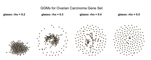
The figure shows how the gene network changes as rho increases. At rho = 0.2, many connections between genes are shown. As rho increases to 0.3 and 0.4, the number of visible connections decreases. At rho = 0.5, most genes appear unconnected, meaning only the strongest relationships are kept. This demonstrates how increasing regularization simplifies the network by filtering out weaker links.
Instead of picking rho by eye, it’s better to use data-driven methods. Cross-validation selects the value that works best on unseen data. The Rotation Information Criterion uses random reshuffling of the data to find a value that avoids adding false connections. The StARS method checks how consistent the network is when using different subsets of the data. The extended Bayesian Information Criterion picks the best network by balancing model fit with simplicity.
These approaches help make sure that the network captures meaningful patterns in the data, such as relationships between genes in ovarian cancer, without being too noisy or too empty.
Conclusion
Gaussian Graphical Models (GGMs) are powerful tools for exploring direct relationships between variables in complex biological data. As omics technologies generate increasingly large datasets, GGMs help simplify these by highlighting which variables are directly connected, rather than just broadly associated. Estimating a GGM requires careful steps, including choosing how much to simplify the network and addressing uncertainty in the results. The authors have shown that a complete GGM analysis can be done using accessible, open-source tools in R, but also emphasizes the importance of thoughtful decision-making in every step, from data preparation to model selection and visualization. As data grows in size and complexity, GGMs remain a valuable approach for uncovering meaningful patterns, and new methods continue to expand their potential in modern biological research.