
Title: A Practical Guide to Selecting Models for Exploration, Inference, and Prediction in Ecology
Author(s) and Year: Andrew T. Tredennick, Giles Hooker, Stephen Ellner, Peter B. Adler, 2021
Journal: Ecology, open access: https://esajournals.onlinelibrary.wiley.com/doi/10.1002/ecy.3336
A statistical toolbox in some ways is like an endless buffet. There are tons of statistical methods out there, ranging from linear models to statistical tests to neural networks. In addition, with increasing amounts of data, new applications from other fields, and increased computational power, methods are constantly being created or improved upon. Having so many possibilities, of course, has its perks. But researchers inevitably must face this daunting question: what method do you choose and why?
In their paper, Tredennick et al. claim that there are three primary goals for statistical modeling in ecology: exploration, inference, and prediction. Exploration is the process of finding patterns in data and creating scientific hypotheses. Inference is the process of assessing whether data supports a hypothesis, and prediction refers to the ability to make accurate predictions for future data. You may be wondering, “Aren’t all of these goals related?” The answer is yes. However, conducting a statistically-sound analysis that accomplishes all three tasks is no easy feat. Tredennick et al. present a case study that highlights how even when using the same data set, each goal involves a nuanced analysis that can lead to different models and results.
The Case Study
This case study considers a data set from Roland and Matter, which consists of yearly population growth rates for 11 different butterfly sub-populations (more specifically, Parnassius smintheus) from 1995 to 2014. In addition, there are measurements for 90 different weather-related independent variables. Some examples are the maximum temperature for each month of the year, the minimum temperature for each month of the year, etc. The authors conducted three separate analyses, one for each goal.
Analysis 1: Exploration
The authors first explored which weather-related variables show a significant association with the population growth rate. To start, they screened out any independent variables, also called covariates, that seemed to have no association with the population growth rate. Then, for each of the remaining covariates, the authors conducted a likelihood ratio test, a commonly used statistical test that measures how “likely” it is for a data set to have come from one model vs. another. Here, the two models of interest are a model which includes all the covariates, and an alternative model which does not contain the covariate of interest. The likelihood ratio test returns a p-value, which is a measure of how much your data supports your hypothesized model. In this case, when the p-value is small, this suggests that the covariate of interest is significant and important to include. In the end, the authors found eight significant covariates which suggested that temperatures in late fall, early winter, and spring had the most notable associations with the population growth rate. One word of caution is that data sets often have patterns by random chance. For example, if you test 100 covariates and use a p-value threshold of 0.05 for each likelihood ratio test, then approximately 5 out of the 100 covariates will come back as significant, but not be significant at all. This phenomenon is called multiple testing and is one reason why researchers should avoid drawing inferences from exploratory data analysis.
Analysis 2: Inference
Next, the authors chose to investigate the following hypothesis: extremely high temperatures in winter affect the population growth rate in years of low snowfall. Here, we pretend that we do not know the results from the previous analysis. The authors first built a model that incorporated four main covariates: level of snowfall, the average maximum temperature in winter, the population size in the previous year, and an interaction term that multiplies snowfall by the average maximum temperature in winter. Because the null hypothesis is about the effect of temperature, paired with low snowfall, on the population growth rate, the authors were primarily interested in the interaction term which utilizes both pieces of information. More specifically, they wanted to test if the interaction term was important to include in the model. Like before, they performed a likelihood ratio test to compare the model with the interaction term to the model without and found that the term was significant. Thus, the results suggest that there is a relationship between snowfall, extremely high winter temperatures, and population growth rate. Comparing this analysis to the previous one, note that here, the authors do not make any conclusions on the significance of spring temperatures. In fact, they do not consider them at all!

Figure 1: This is a plot of mean maximum temperature in early winter vs. population size during low and high snowfall years. Since the relationship between the mean maximum temperature and the population size differs depending on whether there is a high level of snowfall vs. a low level of snowfall, this plot suggests that there could be an interaction effect between the mean maximum temperature and level of snowfall that leads to different trends in population size. Figure 5 in the paper. Figure used under CC BY NC.
Analysis 3: Prediction
Lastly, the authors wanted to generate a model that, given the previous year’s population size and weather information, would yield the best prediction of the population size for the upcoming year. For this analysis, the authors chose to use a Ridge regression model, a variation on the linear regression model. A natural question is “Why Ridge regression?” When fitting a linear regression, we aim to minimize the differences between the observed data and the predictions from the fitted model. However, we also do not want a model that fits the data too closely. When this occurs, you run the risk of also modeling the synchronicities of that data set that occur by random chance instead of just the general trend. As a result, this model may make poor predictions for future data. In Ridge regression, an extra term is added in this minimization problem, called a regularization term, to help deter this phenomenon.
To evaluate predictive performance, the authors used a method called validation. When conducting validation, we split the data into two groups – training and test. We first use the training data to generate the model, and then we apply our model to the test data. We can create predictions and compare them to observed values from the data set. This process allows us to approximately assess how well our model generates predictions for new data.
The authors created an optimal Ridge regression model and compared it to another model that only included the four covariates from the inference analysis. When comparing the predictive performance between the two, the authors found that the former model performed much better, despite the latter’s use of information gained through inference. This highlights that our “best” model in inference is not always our “best” model in prediction.
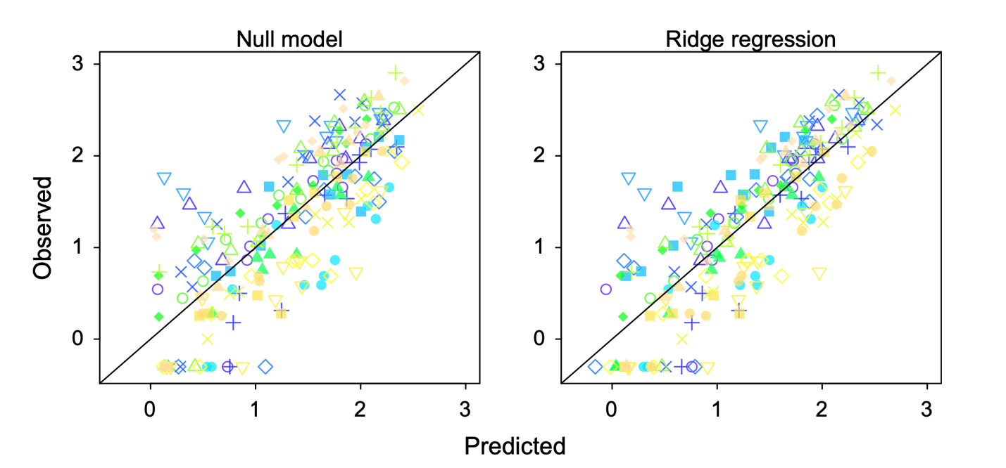
Figure 2: These are scatter plots of predicted population size vs. observed population size. The closer the points are to the black line, the closer the prediction is to the observed value. The plot on the left-hand side plots predictions generated by a model that does not have any weather-related variables. The plot on the right-hand side plots predictions generated by a Ridge regression model that incorporates eight weather-related covariates. Figure 6 in the paper. Figure used under CC BY NC.
The Takeaway
So what is the takeaway? Researchers need to specify the goal of their analysis and the critical thinking behind all their choices. Each data set is a unique snowflake with its own characteristics. In addition, not all statistical techniques are appropriate for each goal. While it is tempting to use one data set to simultaneously investigate all three of the previously stated goals, one must proceed with caution to avoid misinterpreting results and/or reporting false discoveries. By encouraging the best practices laid out in their paper, the authors hope to clear up the confusion surrounding the model selection and bring some transparency to this “black box” process.