
Title: A Simplified Formulation of Likelihood Ratio Confidence Intervals Using a Novel Property
Authors & Year: Necip Doganaksoy (2021)
Journal: Technometrics [DOI: 10.1080/00401706.2020.1750488]
Likelihood Ratio Confidence Intervals
For statistical modeling and analyses, construction of a confidence interval for a parameter of interest is an important inferential task to quantify the uncertainty around the parameter estimate. For instance, the true average lifetime of a cell phone can be a parameter of interest, which is unknown to both manufacturers and consumers. Its confidence interval can guide the manufacturers to determine an appropriate warranty period as well as to communicate the device reliability and quality to consumers. Unfortunately, exact methods to build confidence intervals are often unavailable in practice and approximate procedures are employed instead. Traditionally, confidence intervals based on the asymptotic normal distribution of the maximum likelihood estimators (MLE) have gained widespread popularity due to their simplicity and ease of computation. However, the resulting confidence intervals can be highly inaccurate for small samples as they are based on the large sample theory (i.e., asymptotics). The approximate chi-square distribution of the likelihood ratio test (LRT) statistic provides an alternative method to obtain confidence intervals. For a wide class of models, LRT-based confidence intervals have been shown appreciably more accurate than the asymptotic normal confidence intervals. The LRT-based methods provide a flexible and unified framework to accommodate special kinds of models and type of data (e.g., nonnormal and skewed probability distributions, truncated models, incomplete data due to censoring, etc.) that are often encountered in practice.
How to Compute LRT-based Interval – Old Way
For anyone who has taken an undergraduate course in mathematical statistics, it is a well-known fact that for large samples, the LRT statistic is approximately distributed as a chi-squared random variable with one degree of freedom. The problem is that closed-form solutions for the LRT-based confidence limits are typically not available and so, one must employ numerical methods to find the lower and upper limits of a confidence interval. Conventionally, the solution is obtained in two stages. In the outer search over a confidence limit (say, the upper limit θU for example), the log-likelihood is first maximized with respect to the nuisance parameters λ (e.g., the standard deviation of a normal distribution), given a value of the parameter of interest θ (e.g., the mean of a normal distribution). It is called the profile log-likelihood and its computation may require a multi-dimensional optimization since the dimension of λ could be more than one. Figure 1 (a) provides an illustration of an outer search over θ in k steps, where the green dot represents the location of the global MLE. The arrows trace the trajectory of the profile log-likelihood until we find a range of θ containing the contour at level k. The constant k can be regarded as a horizontal slicer of the log-likelihood to produce a contour at a desired confidence level (say, 95%). Once this range of θ is found, the inner search then starts, where a one-dimensional root-finding procedure is implemented to find the exact point θU at which the profile log-likelihood equals the set value k; see the red dot in Figure 1 (b). The iterative process to find the lower limit θL is also similar. As seen, this two-step algorithm is cumbersome and can be computationally expensive and time consuming. This is the reason why the LRT-based confidence interval is not so popular in practice.
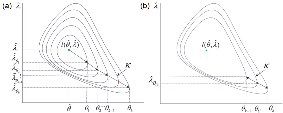
Figure 1. Contour plot of the log-likelihood and illustration of the
conventional approach to find the upper confidence bound θU
How to Compute LRT-based Interval – New Way
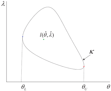
This work proposes a simplified and intuitively appealing algorithm by exploiting an overlooked property of the log-likelihood function. That is, the lower (upper) confidence limit can be found by directly minimizing (maximizing) a contour of the log-likelihood at a desired level without going through explicit evaluations of the profile log-likelihood. By removing calculation of the constrained MLE of nuisance parameters, this transforms the two-step procedure into a single-step procedure, which is a traditional nonlinear constrained optimization problem. Figure 2 presents a schematic based on the novel property that defines the confidence limits without any explicit reference to the corresponding values of a nuisance parameter λ. The proposed method lends itself to a straightforward solution through standard optimization features that are widely available in commercial and open-source software (e.g., the gosolnp function of the R package Rsolnp).
Computational Advantage & Practical Benefits
The study presents two case studies for illustration based on applications in product quality and reliability improvement. The first study is about interval estimation for the difference between the averages of two log-normal populations, motivated by reliability assurance in semiconductor manufacturing, while the second is about interval estimation for misclassification probabilities attributable to measurement error of a thermoplastic resin extruded in batches, which is used to make various plastic products such as toys and bottles. When compared to the conventional approach, the proposed method was found most compelling when the function of parameter(s) is not invertible because it resulted in substantial savings of computational time. It is noted that implementation of the proposed approach requires a robust algorithm for nonlinear constrained optimization. That is, the algorithm must be able to find the optimal point regardless of the problem setup. Nowadays, such algorithms are readily accessible to practitioners who do not necessarily possess an in-depth knowledge of numerical optimization methods. Thus, it is expected that the method can be successfully applied in a wide variety of inferential problems of quality and reliability assessments that include lifetime data with multiple failure modes, mixture models for limited failure populations, accelerated life testing, accelerated degradation testing, etc. For instance, a manufacturer can estimate the average lifetime of a newly designed cell phone, and the method discussed here can be used to construct its confidence interval in order to assess the quality and reliability of the new product before it is released to the market and sold to consumers.