
Complex polynomials are one of the oldest and most fundamental objects of study in mathematics, and are ubiquitous in applications. A complex polynomial is a mathematical expression of the form
where d is a fixed natural number (like 1, 2, 3, . . .), ad, . . . , a0 are complex numbers, and z is a variable that takes values in the complex numbers. (Recall that a complex number is a number of the form a + bi where a, b are real numbers and i =√−1.
We say that d is the degree of the polynomial and ad, . . . , a0 are the coefficients. Every polynomial can be factored into the form
where r1, . . . , rd, called the roots, are complex numbers. If we plug in any root r1 to the polynomial we get 0, so we also call the roots the zeroes of the polynomial. We can see that every polynomial can be specified by the (ordered) list of d + 1 coefficients or specified by the (unordered) list of d roots. We can visualize complex functions in the following way: we assign a color to every point on the complex plane. Then we plot a function f(z) by coloring the point z by the color assigned to the point f(z). See Figure 1.
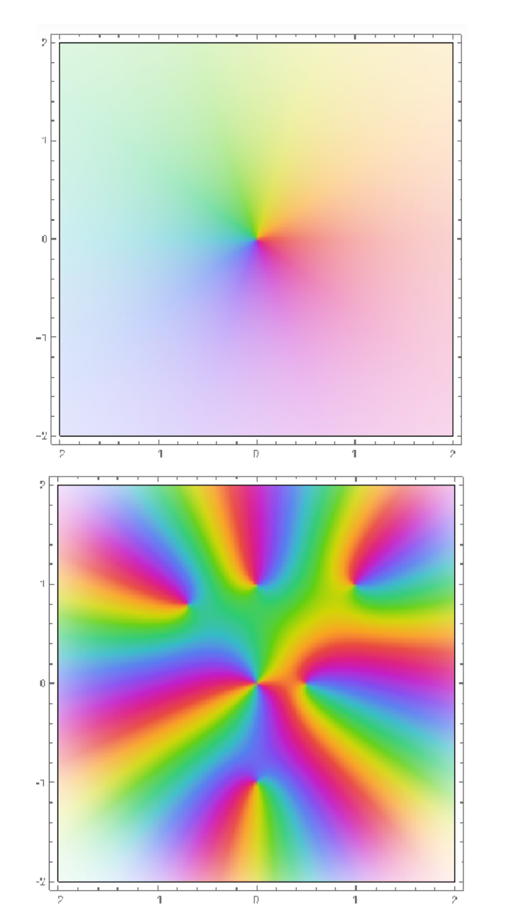
Figure 1: The top image shows the color assigned to each point in the subregion of the complex plane where the real and imaginary components are both between −2 and 2. The bottom figure is the plot of a complex polynomial. The black dots correspond to the zeroes of the complex polynomial.
One result dating back to the 19th century relates the location of the zeroes of a polynomial to the critical points, which are the zeroes of the derivative of the polynomial. The Gauss-Lucas theorem essentially says that if you play connect-the-dots with the zeroes of a complex polynomial, the critical points will lie within the resulting figure. See Figure 2 for an example.
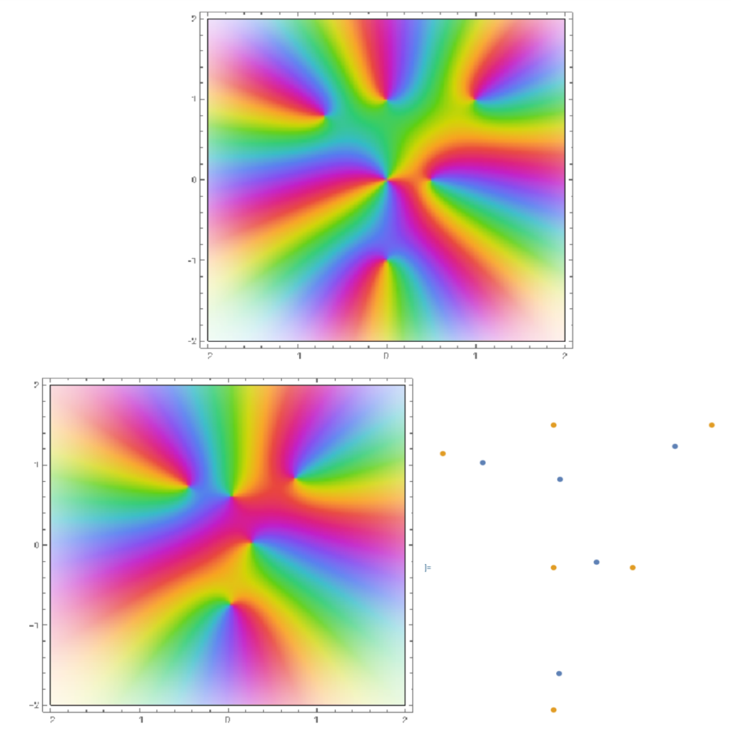
Figure 2: The top image is the plot of the polynomial, and the bottom left image is the plot of its derivative. The bottom right image shows the relationship between the zeroes of the polynomial (yellow dots) and the zeroes of the derivative (blue dots)
Here are two physical interpretations of this phenomenon:
- Suppose that for each root of the polynomial, we place an electric point charge of equal charge on the corresponding point of the complex plane. Then the critical points are the points of equilibrium in the resulting force field.
- Suppose fluid is flowing into the complex plane from the roots of the polynomial. Then the critical points are the stagnation points (the points where the water is not moving) in the resulting two-dimensional flow.
Thus we can see how polynomials may be useful in the study of physical systems. In practice when studying large physical systems, we often prefer to deal with the statistics of the system then trying to track the behavior of individual particles. For example, if we put a drop of food coloring into a glass of water and then stir, it would be very hard to model where each individual food coloring particle ends up within the cup at the end of the process. On the other hand, we can predict that the entire collection of food coloring particles will be uniformly distributed throughout the water. Along these lines, it can be interesting to study the properties a polynomial is statistically likely to have when we introduce random parameters to the polynomial. This was studied in the recent paper: ”Zeros of Random Polynomials and Their Higher Derivatives.” This paper extends previous results on critical points by studying the properties of higher derivatives of random polynomials. Just like how the critical points may correspond to the points in a fluid flow with no velocity, the zeroes of higher derivatives will correspond to points of the fluid flow where there is no acceleration, jerk, etc, which are quantities that have physical meaning.
One way to introduce randomness into a model is to choose the roots of the complex polynomial independently at random according to a probability measure, which is a function that assigns to each region of the complex plane the likelihood that a root will be chosen from that region. The authors prove that for a given probability measure, if we choose a sequence of polynomials of increasing degree according to this scheme, the distribution of the roots of each higher derivative converges to the original probability measure. There is some subtlety here: if the distribution of the roots converges to a certain probability measure, it is not true that the critical points necessarily converge to the same probability measure. To see this one can think of placing charges (i.e. the roots) at equal distances from one another around a circle centered at the origin. The equilibrium (i.e. the critical point) of the resulting force field will always be at the origin, not on the circle. Therefore to obtain the conclusion in the result we need to know more than the probability measure of the roots; the way we choose the roots according to the probability measure matters as we can see in the above example.
The authors then apply their results when the zeros of the random polynomials follow the density of the 2-dimensional Coulomb gas ensemble. This means that the zeros of the polynomial correspond to the locations of electrons of the complex plane which are being influenced by an external field. The measure of the system is a function which for each region of the complex plane outputs how many electrons are in that region. The authors are able to say that the distribution of zeroes of higher derivatives of the polynomial with roots describing the locations of the electrons at equilibrium converge to distribution of the electrons at equilibrium. We can interpret this finding as saying that there are no ”special” places that points of the system with ”special properties are likely
to be in within the larger system.