“Changes” in statistics, “changes” in computer science, changes in outlook

Moinak Bhaduri
Bentley University, Math Sciences

No matter how free interactions become, tribalism remains a basic trait. The impulse to form groups based on similarities of habits – of ways of thinking, the tendency to congregate across disciplinary divides, never goes away fully regardless of how progressive our outlook gets. While that tendency to form cults is not problematic in itself (there is even something called community detection in network science that exploits – and exploits to great effects – this tendency) when it morphs into animosity, into tensions, things get especially tragic. The issue that needs to be solved gets bypassed, instead noise around these silly fights come to the fore. For example, the main task at hand could be designing a drug that is effective against a disease, but the trouble may lie in the choice of the benchmark against which this fresh drug must be pitted. In popular media, that benchmark may be the placebo – an inconsequential sugar pill, while in more objective science it could be the drug that is currently in use. There are instances everywhere of how scientists and journalists come in each other’s way (Ben Goldacre’s book Bad Science imparts crucial insights) or how even among scientists, factionalism persists: how statisticians – even to this day – prefer to be classed as frequentists or Bayesians, or how even among Bayesians, whether someone is an empirical Bayesian or not. The sad chain never stops. You may have thought of this tendency and its result. How it is promise betrayed, collaboration throttled in the moment of blossoming. While the core cause behind that scant tolerance, behind that clinging on to, may be a deep passion for what one does, the problem at hand pays little regard to that dedication. The problem’s outlook stays ultimately pragmatic: it just needs solving. By whatever tools. From whatever fields. Alarmingly, the segregations or subdivisions we sampled above and the differences they lead to – convenient though they may be – do not always remain academic: distant to the point of staying irrelevant. At times, they deliver chills much closer to the bone: whether a pure or applied mathematician will get hired or promoted, how getting published in computer science journals should be – according to many – more frequent compared to those in mainstream statistics, etc.

Of late, people have noted the frequent pointlessness of these fights and attempts are underway to look at commonalities: Deepak Chopra and Leonard Mlodinow’s book War of the Worldviews: Where Science and Spirituality Meet — and Do Not is a great example or Chen’s (2019) work on how computer scientists and statisticians approach a well-known classification method – the k-nearest neighbor (knn), if you’d prefer unification with a narrower spectrum. The article we are discussing, Automatic Change-Point Detection in Time Series via Deep Learning by Jie Li, Paul Fearnhead, Piotr Fryzlewicz, and Tengyao Wang documents yet another happy coming together of two fields that are, at times, perceived to be at odds or to be guided by different motivations: statistics and computer science. Statistics raises the problem; computer science helps furnish an answer and in turn, gets enriched. It’s all about change-points. Finding where exactly, and if possible, why exactly, substantial shifts happened in the nature of an incoming data stream. And just as the drug benchmarks above may be installed through mainstream media or through science, or just as knns may be appreciated in two different ways, these shifts – as we shall see – may be detected through tricks from both statistics and computer science.

The importance of change-finding 

We will get to the main article in just a moment. Let’s spend some time grasping what change points are and what good they are. Although a great exercise in itself, you may not be strictly interested in knowing where changes – that is where, in a chain, substantial deviations from the current trend – happened. Oddly, it has this habit of cropping up in other contexts when you least expect it to – contexts that you might be interested in. Here’s a quick experiment. Imagine some events happening at these times measured with some grand clock that measures time from some grand origin of $0$:

$0.5, 1.5, 2.5, 3.5, 4.5, 5.5, 5.75, 6.00, 6.25, 6.50, \textcolor{blue}{\{6.75, 6.85, 6.95, 7.05\}}$

These events could be anything: times at which earthquakes happened, times at which COVID-19 patients got admitted to hospital, anything at all. Imagine not having seen the last four times shown in blue (technically, the test set) and having to predict the number of events within the half unit period post-6.5. The hospital may need to make provisions for beds, for instance. 

$0.5, 1.5, 2.5, 3.5, 4.5, 5.5, \textcolor{red}{5.75, 6.00, 6.25, 6.50,} \textcolor{blue}{\{6.75, 6.85, 6.95, 7.05\}}$

Notice the increased rate of events post-5.75. If you hadn’t noticed this, and if the forecasting tool you had was simple: calculating the number of events per unit time and multiplying that rate by the time horizon, your guess would have been $\frac{10}{6} \times 0.5 = 0.83$ or about $1$ – far away from the real answer of 4. In contrast, if you had calculated the rate on the region of upped activity shown in red – on the relevant history, so to speak – and done the same thing, your answer would have been $\frac{4}{6.5-5.75} \times 0.5 = 2.67$ or about $3$ much closer to the actual value. Similar things happen if your tool gets more sophisticated than simple rates and multiplication. $5.75$ is called a change-point or a break-point: it marks the onset of a fresh rate and the process of discovering these types of points – through checking whether the rate difference is substantial enough – is called change-detection or change-point analysis. Your main goal was not discovering $5.75$; it was just forecasting. But the change-point came in the way; it bettered the analysis: $3$ is much closer to $4$ than $1$ is.

Historically, these break-points have been located through tools called “control charts” – much like the one shown in Fig. 1 below. These tools, introduced by Shewhart, Page and others (a detailed history in Montgomery (2005)) are quite popular in statistical quality control. They have two pieces: a “central line”, shown through the solid horizontal line in Fig. 1 which depicts some ideal scenario what would happen to functions calculated from a time series had it been extremely well-behaved and devoid of variation, and a pair of “control limits” which tells one how much oscillating from this ideal scenario is okay. The idea is simple: each time an observation from a time series comes in, one computes a statistic – maybe the running average of inter-event times over the last three points, and places it along the vertical axis of this chart. If it falls within the allowable range of variation – like the first four green values did on Fig. 1 – the fluctuations are taken to be due to random chance: noise that you would expect anyway. If, however, one falls outside – like our fifth red point did, the deviation is deemed substantial enough to suspect the cropping up of a change-point at that location. Simple though it may sound, the strategy has limitations. The upper and lower control limits are placed assuming many things: the kind of change one is looking for, the distribution of the values one is plotting etc. For instance, if one were interested in detecting changes in an average, the limits would be different than those if one were to detect shifts in a variance. Each control chart is restricted to a context, each to certain assumptions. And those assumptions may be difficult to check a priori. It is at such times of strict restrictions, restrictions that keep changing, that we crave sensibilities attuned to the changeless. Precisely what the authors – through borrowing ideas from neural networks – offer.

The main magic: recognizing the CUSUM (from statistics) – neural network (from computer science) equivalence 

The authors are honest up front: the methods they offer are for offline detection – that is, when one looks back at the full and frozen history and tries to pinpoint a structural break, as opposed to an online detection where one is tasked with saying whether an incoming observation is a change-point, in a continuous fashion, that is. But that’s no major limitation. The literature is littered with examples where offline tools are upgraded to become online tools with a few predictable tricks. Our authors begin by looking at an established way of detecting changes in a discrete time series, that is in a series much like the one we encountered in the previous section, through the Cumulative Sum (or, affectionately, the CUSUM) function which is quite well-known in statistics (Montgomery (2005)). Given a sequence $X$, this function wants us to keep a running record of the distances between a possible pre-change piece of $X$ and the corresponding post-change piece, treating each time point as a potential change-point candidate, through a function $C(X)$, the $C$ standing, typically, for the cost. If at any point this difference – this gap – becomes too big, i.e., if it exceeds a threshold $\lambda$, one may reasonably suspect the presence of a change-point there. All this is formalized through the CUSUM statistic:

$$ h_\lambda^{\text {CUSUM }}=1\{||C(X)||>\lambda\} .$$

We are plotting, therefore, $C(X)$ along the vertical axis of Fig. 1 and specifies the wiggle-room around the central line. The authors also recall a structure quite familiar in computer science: neural networks – a typical one shown in Figure 2 (Li, J, Fearnhead, P, Fryzlewicz, P, Wang, T. (2024)) below.

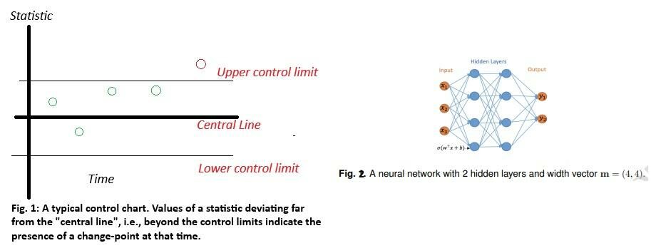
With many details and information entering the input nodes on the far-left, the structure mashes them up through the intervening hidden layers and outputs through the two (at least, for now) output nodes results you may be interested in: the chances of someone having good or bad credit, for instance (or, in our case, of saying whether a point is a change-point or not). Call such a structure $h(x)$ and imagine a bag called $\text{H}_\text{L,m}$ that stores such kind of structures with L hidden layers and a width vector m. This width vector says how many hidden nodes you have in each hidden layer. Like in figure 1, $L = 2$ and $m = (4,4)$.

That sounds profound! But what use is that discovery?

It’s immensely useful, actually! In statistics, there are many tools, not just the CUSUM, that detect changes. The trouble is most, if not all, are context-specific: i.e., the type of change one is trying to catch, matters. The CUSUM, for instance, is good at nabbing changes in a time series average (in case the noise – the fluctuations – are normally distributed). Others are good at detecting changes in variance, or in other specifics about the shape of the underlying probability distribution generating the values, etc. Because the $\text{H}_\text{L,m}$ bag contains many neural networks, the authors claim and document, crucially, through simulations, how some element of this bag, some specific neural network, that is, will always deliver great detection performance, whatever the type of change it is you are worried about. Be it changes in a mean, a variance, or anything else. You do not need to nitpick. And yet, you are still assured of a better detection accuracy – better than the established options such as the CUSUM. The two-way bridge spawns not just one, but a collection of classifiers (or, detectors, now that they are the same), some of which should work out (in terms of accuracy, delay times, etc.) no matter the context. The article we looked at brings out a construction-based limitation of mainstream statistical change-detection methods (the need to stay tethered to the context) and in so doing, points to an encouraging unity between that class of tools and neural networks. You may rightly question: why the obsession with neural networks? They need lots of data, and I thank my writing buddy David Han, who pens excellent quality control pieces here, for pointing this out. There are loads of classifiers that do what they are supposed to do: classify! Random forests, k-nearest neighbors, etc. The authors point out those could be fruitful avenues for future work. In the admirable spirit of reproducibility, they’ve made their codes public too. Collectively, they’ve shown how staying curious about an object – a tool (i.e., neural networks in this instance) – one doesn’t normally deal with while addressing a specific problem (change-point detection), can forge an immensely useful connection. Each, housed within a non-computer science department, has demonstrated how a frank open-mindedness could instill a slight tingle of optimism, triggering an insight truly worthy of a wow.

References

Goldacre, B. (2009). Bad Science. HarperPerennial.
Chopra, D., & Mlodinow, L. (2011). War of the worldviews: science vs. spirituality. New York, Harmony Books.
Chen. H. (2019) “Sequential change-point detection based on nearest neighbors.” Ann. Statist. 47 (3) 1381 – 1407, https://doi.org/10.1214/18-AOS1718
Li, J, Fearnhead, P, Fryzlewicz, P, Wang, T. (2024) Automatic Change-Point Detection in Time Series via Deep Learning, Journal of the Royal Statistical Society Series B: Statistical Methodology, https://doi.org/10.1093/jrsssb/qkae004
Montgomery, D. (2005). Introduction to Statistical Quality Control. Hoboken, New Jersey: John Wiley & Sons, Inc. ISBN 978-0-471-65631-9. OCLC 56729567. Archived from the original on 2008-06-20.
Schmidt-Hieber, J. (2020). Nonparametric regression using deep neural networks with ReLU activation function. Ann. Stat. 48 (4), 1875–1897
Bhaduri, M (2018), “Bi-Directional Testing for Change Point Detection in Poisson Processes”. UNLV Theses, Dissertations, Professional Papers, and Capstones. 3217. http://dx.doi.org/10.34917/13568387