
Title: Sequentially Valid Tests for Forecast Calibration
Authors and Year: Sebastian Arnold, Alexander Kenzi, and Johanna F. Ziegel (2023)
Journal: To appear in Annals of Applied Statistics
The meteorologists of today no longer ask themselves, “Will it rain tomorrow?”, but rather, “What is the probability it will rain tomorrow?”. In other words, weather forecasting has evolved beyond giving simple point projections, and instead has largely shifted to probabilistic predictions, where forecast uncertainty is quantified through quantiles or entire probability distributions. Probabilistic forecasting was also the subject of my previous blog post, where the article of discussion explored the intricacies of proper scoring rules, metrics that allow us to compare and rank these more complex distributional forecasts. In this blog post, we explore facets of an even more basic consideration: how can one be sure their probabilistic forecasts make sense and actually align with the data that ended up being observed? This ‘alignment’ between forecasted probabilities and observations is referred to as probabilistic calibration. Put more concretely, when a precipitation forecasting model gives an 80% chance of rain, one would expect to see rain in approximately 80% of those cases (if the model is calibrated).
Forecast calibration is often evaluated using a statistical technique known as the Probability Integral Transform (PIT). Essentially, the PIT is a quantity computed using a distributional forecast for a given time point along with the observed value. When calculated over many time points, we expect these PIT values to follow a uniform distribution for calibrated forecasts. Accordingly, to test calibration, forecasters often employ statistical goodness-of-fit tests for the uniform distribution, which have been a topic of study for many decades. Given a random sample (in this case, the PIT values) and a proposed distribution (e.g., uniform), a goodness-of-fit test attempts to answer the question, “How well does this sample match our expected distribution?” A primary output of these tests is a p-value–a very low p-value gives evidence of inconsistency between the sample and the proposed distribution. In our case, this low value would point to a lack of calibration from our forecasting model.
Although such tests are ubiquitous in the forecast calibration literature, a recent article by Arnold, Henzi, and Ziegel contends that these classical approaches are ill-equipped to truly handle the sequential nature of forecasting. In particular, forecasters often plan experiments to track the performance of their models as new data flows in. Ideally, calibration could be continually monitored each time a fresh observation was recorded, but this violates the assumptions of classical tests for uniformity. Established methods typically require that the sample size is known in advance, thus forcing practitioners to produce forecasts for a pre-specified period of time and wait until all observations have been made before looking at the data. If they want to analyze sub-periods, then this must be planned ahead of time; otherwise, the resulting p-values are no longer valid. The authors argue that this fixed sample-size approach can lead to inefficiencies and possible mistaken decisions in the forecasting setting. For example, it may be quickly clear that forecasts are poorly calibrated under a given model, but the classical procedure does not allow for stopping the experiment early without risking the statistical validity of results. Additionally, it might be the case that early forecasts are heavily biased in one direction, but later forecasts switch their bias to the other direction. Hence, at the end of the set observation period, the forecasts may look calibrated, but any analysis of the intermediary periods would soon reveal major flaws in the forecasting methodology.
Therefore, this article argues that a new paradigm should be used for testing forecast calibration, one that respects the sequential nature and allows practitioners to continually monitor forecast calibration as well as stop early if lack of calibration becomes evident. Of course, such a paradigm would still need to formally quantify such evidence for or against calibration, just as p-values do in the classical goodness-of-fit test setting. The proposed solution are quantities known as e-values, which have been a topic of considerable research in recent years. In fact, a seminal work on e-values was the topic of yet another MathStatBites post, and interested readers are encouraged to read Moinak’s summary for details on this innovative inferential concept. From a practical standpoint, there are just a few key ideas to understand the utility and interpretation of e-values. Each forecast + corresponding observation produces an e-value, and these e-values can be easily combined to represent an accumulated body of evidence for or against calibration. If our accumulated e-value is very large (much greater than 1), then we have considerable evidence that our PIT values are not uniform, and thus our model is not calibrated.
The benefit of e-values over the classical methods is perhaps best illustrated graphically. As part of their real-data application, the authors look at wind speed forecasts from an ensemble weather prediction system and analyze their calibration using e-values. Calibration checks for the 24-hour-ahead forecasts at a given station are shown in Figure 1. On the left, we see a histogram for the PIT values over the entire forecasting period (the fixed sample size that a p-value-based approach would test). For a calibrated model, this histogram should have bins with roughly equal heights, and we can see that this particular example actually does look pretty close to uniform. Hence, we might be convinced to call our method calibrated and move on. But then we can look at the right plot, where the accumulated e-values across time are plotted. Around 2012, the e-values are incredibly high, representing considerable evidence that forecasts were definitely not calibrated. This lack of calibration was later ‘washed out’ by later forecasts which were calibrated. Thus, e-values can help the practitioner better identify forecast misspecification, in a way that classical approaches could not due to their incompatibility with sequential observations.
Overall, this novel proposal for testing forecast calibration using e-values provides practitioners new ways to evaluate forecasts in a manner more suited to the ever-evolving nature of time series data. In addition to what has been discussed in this brief summary, the article also includes derivations of e-values for several variations of uniformity tests that arise in different forecasting scenarios and explores the power of different e-value approaches when compared to classical tests that use p-values. Check out the full article, accepted for publication in the Annals of Applied Statistics, for all the technical details and more involved discussion. For those looking to read even more about the intersection of e-values and forecast evaluation, additional articles by Henzi and Ziegel as well as Choe and Ramdas may be of interest.
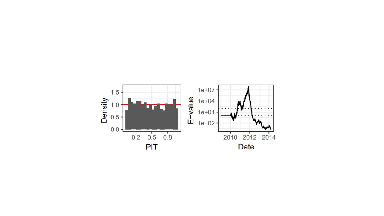
Figure 1: On the left, PIT histogram for 24-hour-ahead forecasts of wind speed at a specific weather station. On the right, e-values for testing uniformity of the PIT, with dashed horizontal lines at levels of 1 and 100. These plots are taken from Figure 4 in the original article.