Title: An Agent-Based Statistical Physics Model for Political Polarization: A Monte Carlo Study
Authors & Year: Hung T. Diep, Miron Kaufman, and Sanda Kaufman (2023)
Journal: Entropy [DOI: https://doi.org/10.3390/e25070981]
Review Prepared by Amal Machtalay
Political polarization refers to a phenomenon where people’s political beliefs become radical, often resulting in the increasing division between political parties, which can have significant social consequences. This polarization is a complex system that is characterized by multiple factors: numerous interacting components (individual agents/voters, politicians, groups, media, etc.), non-linear dynamics (meaning that small changes can lead to large and uncertain effects), and emergent behavior (where collective phenomena result from local interactions, like when individuals engage with posts on social media that align with their political beliefs).
The authors study the case of three USA political groups, each group indexed by $i\in \left\{ 1,2,3\right\}$:
- Group 1 ($i=1$) represents Democrats who identify as progressives.
- Group 2 ($i=2$) represents Republicans who identify as conservatives.
- Group 3 ($i=3$) represents Independents who identify as unaffiliated.
Two types of interactions are classified and illustrated in Figure 1:
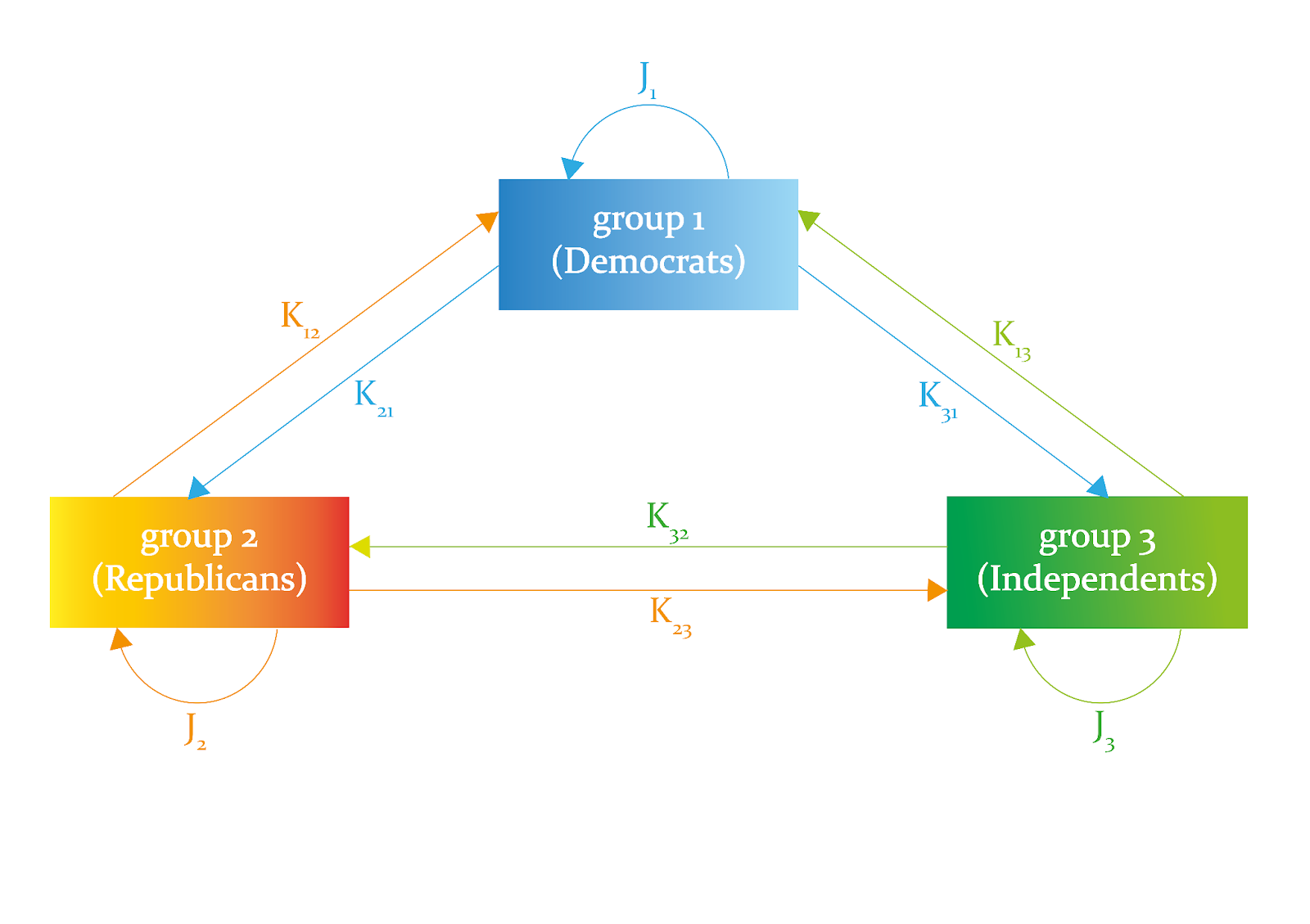
Figure 1: A schematic of intra-interactions ($J_1, J_2, J_3$) and inter-interactions ($K_{12}, K_{21}, K_{23}, K_{32}, K_{13}, K_{31}$) between three political groups: Democrats, Republicans and Independents (Adapted from Diep HT et al., Figure 1).
- Intra-group interactions denoted by $J_i$ which quantifies the cohesiveness of group $i$, indicating the degree of unity, trust, and solidarity among its members. The authors consider a specific case for their study, where the Democrats are considered more cohesive than the Republicans ($J_1 > J_2$). Independents, by definition, do not adhere to a unified political framework and therefore have no cohesion ($J_3=0$).
- Inter-group interactions denoted by $K_{ij}$ which quantifies the effect of group $i$ on group $j$.
$K_{ij}> 0$ → Attraction of group $i$ toward group $j$
$K_{ij}< 0$ → Resistance of group $i$ toward group $j$
$K_{ij}= 0$ → No influence between group $i$ and group $j$
Parameters $J$ and $K$ are determined quantitatively using publicly available poll data. To elaborate this data, the statisticians survey people who are randomly selected to represent every political group. Once the answers are collected, they are analysed and interpreted, then finally presented to the public as reports, charts, and graphs.
Each $i$’s group member, indexed $m$, has a stance at time $t$ denoted by $S_i(m,t)$ in [-1,1], representing their position on the political continuum [-1,1], which is a scale from a strong left political stance (-1) to a strong right political stance (+1). Individuals in each group $i$ align their stances with the mean stance of the group denoted <$S_i$>. Where<$S_1$> → -1 (Democrats/left position),<$S_2$> → +1 (Republicans/right position), and<$S_3$> → 0 (Independents/no position). For instance, consider within Democrats ($i=1$) that there are three members indexed as $m=1, m=2, m=3$, where at a specific time $t$, their political stances are: $S_1(1,t)=+0.7, S_1(2,t)=+0.5, S_1(3,t)=+0.8$. In this case, the mean stance

The individual $m=1$ with a stance of $+0.7$ would align closely with the group’s average position.
Each group $i$ has a leader who has an effect on their group members. The effect is represented by a magnetic field denoted $h_i$, where:
$h_i>0$ → <$S_i$> is shifted toward positive values
$h_i<0$ → <$S_i$> is shifted toward negative values
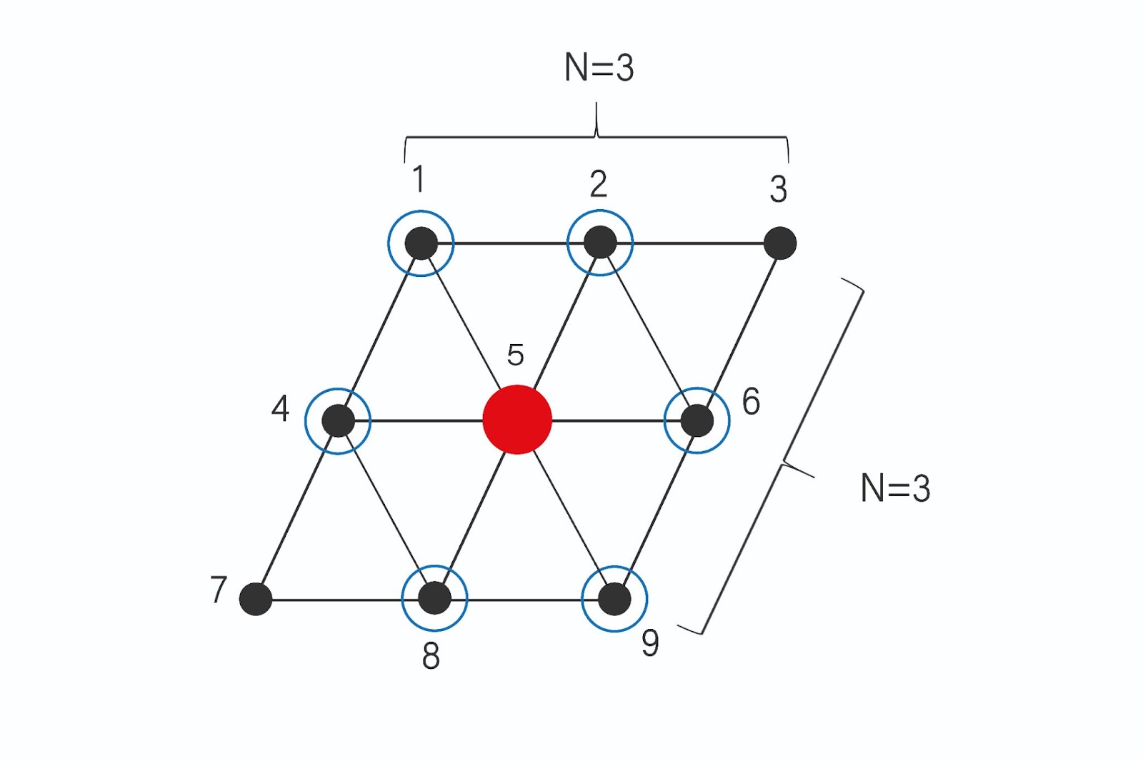
In order to gain a deeper understanding of group dynamics and how they influence the overall system behavior, the authors examine short-range intra-group interactions. To conceptualize these interactions, every group $i$ is represented by a triangular lattice of size $N$ × $N$ (for instance, $N=3$), as illustrated in Figure 2, where each node corresponds to a group member $m$ ($m=1,2,3,4,5,6,7,8,9$) that interacts exclusively with their nearest neighbors $nn$ (six at most) with whom they are generally in contact. For instance, the nearest neighbors of the red node ($m=5$) are the six nodes circled in blue ($m=1,2,4,6,8,9$), while the node indexed $m=7$ has only two nearest neighbors ($m=4,8$). This type of interaction model is referred to in the literature as an Agent-based model.
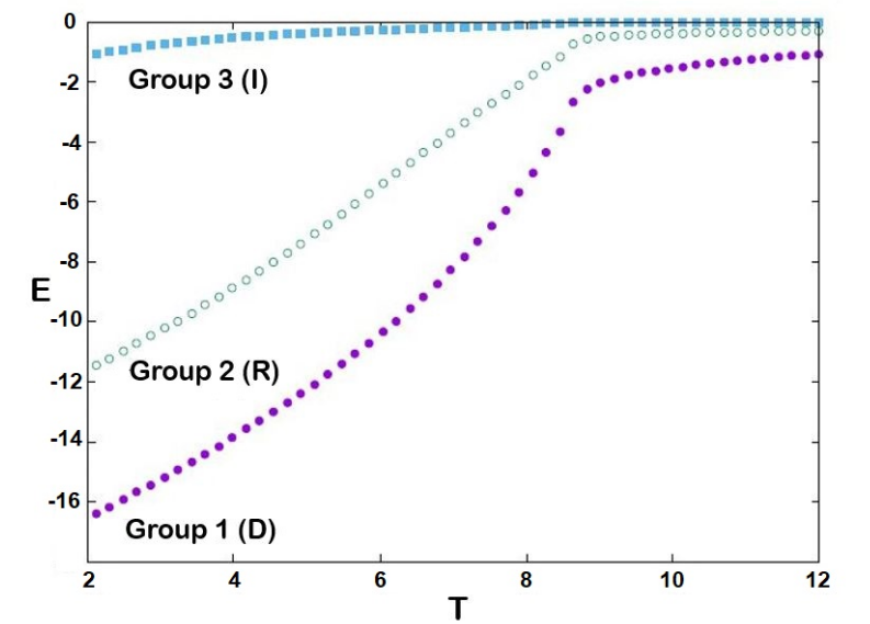
Two other important parameters are borrowed from the field of Statistical mechanics (which provide insights into the thermodynamic characteristics, phase transitions, and behaviors of substances at different scales). The first one is what the authors named political temperature denoted $T$, which represents the political ambience of the society. For example, during elections or politically tense times, the $T$ is large, otherwise it is low. The second parameter is the interaction energy denoted $E_i(T)$ which illustrates the political state of the group $i$, influenced by the political temperature $T$. For instance, if individuals within the group $i$ share similar opinions, the interaction energy between them would be high. Conversely, if individuals have opposing views, the interaction energy might be low, indicating a lack of agreement.
$E_i(T)=(<H_i(T)>)/{N^2}$
$H_i(t)$ is defined as the Hamiltonian of group $i$ at time $t$ that involves all interactions. It is made up of three terms. The first term represents the intra-group interactions, which are involved over the nearest neighbors nn ($p$ and $q$) within group $i$. The second term indicates the effect of the leader on all the members of group $i$. The last term represents the inter-group interactions (the interactions of group $i$ with the average stances of the other groups $j$ at $t-1$).
To illustrate $H_i(t)$ in a simple example, let’s imagine again that there are 9 members in group 1 represented in Figure 2 as a lattice of size 3 × 3, where at time $t$, their political stances are considered in Table 1. Each member has at most six nearest neighbors ($nn$) as shown in Table 1.
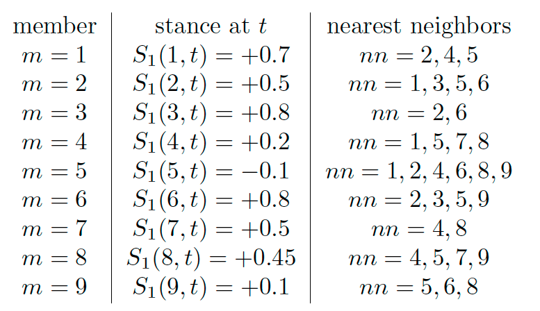
Table 1: An example of the political stance at $t$ and the nearest neighbors for each member in group 1.
Assume, the average stances of groups 2 and 3 from the previous time step ($t-1$) are <$ S_2(t-1)$>$ =-0.5 $ and <$ S_3(t-1)$>$ =-0.1$ respectively. We consider $J_1=5, h_1=1, K_{12}=-4$ and $K_{13}=0$.
Based on the Hamiltonian equation provided earlier, we have the first term equal to -21.35, the second term is equal to -3.95, and the third term equal to =-7.9. Then, $H_1(t)=(-21.35)+(-3.95)+(-7.9)=-33.2$. The negative sign in the Hamiltonian function implies an attractive interaction between individuals within the same group. It indicates that the system tends to lower its energy in order to reach equilibrium (stabilize).

Hence <$H_i(T)$>=(∑_{t_1}^{t_2} H_i(t))/(t_2-t_1)$.
For example, consider a second time step for the example in Table 1 where $H_i(1)$ is what we calculated above and, H_i(2)=-30, then <$H_i(T)$>$=(H_i(1)+H_i(2))/(2-1)=(-33.2-30)/(2-1) =-31.6$ . Therefore, $E_i(T)=(<H_i(T)>)/{N^2}=(-33.6)/(3^2)=-3.73$. This kind of operation enables us to follow the political state of each political group $i$ over time by computing their interaction energy $E_i(T)$ within different political temperatures $T$ as showcased in Figure 3, where the specific political temperatures at equilibrium, called the transition temperature (where the interaction energy is the lowest), is denoted for each group as $T_1, T_2$, and $T_3$ (approximately $8.6, 8.5$, and $8.4$ respectively).