Data Fission – Statistical Analysis through Data Point Separation
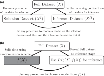
Title: Data Fission: Splitting a Single Data PointAuthors & Year: J. Leiner, B. Duan, L. Wasserman, and A. Ramdas (2023)Journal: Journal of the American Statistical Association[DOI:10.1080/01621459.2023.2270748]Review Prepared by David Han Why Split the Data? In statistical analysis, a common practice is to split a dataset into two (or more) parts, typically one for model development and the other for model evaluation/validation. However, a new method called data fission offers a more efficient approach. Imagine you have a single data point, and you want to divide it into two pieces that cannot be understood separately but can fully reveal the original data when combined. By adding and subtracting some random noise to create these two parts, each part contains unique information, and together they provide a complete picture. This technique is useful for making inferences after selecting a statistical model, allowing for better flexibility and accuracy compared to traditional data splitting…
Unveiling the Dynamics of Human-AI Complementarity through Bayesian Modeling
Article Title: Bayesian modeling of human–AI complementarity Authors & Year: M. Steyvers, H. Tejeda, G. Kerrigan, and P. Smyth (2022) Journal: Proceedings of the National Academy of Sciences of the United States of America [DOI:10.1073/pnas.2111547119] Review Prepared by David Han Exploration of Human-Machine Complementarity with CNN In recent years, artificial intelligence (AI) and machine learning (ML), especially deep learning, have advanced significantly for tasks like computer vision and speech recognition. Despite their high accuracy, these systems can still have weaknesses, especially in tasks like image and text classification. This has led to interest in hybrid systems where AI and humans collaborate, focusing on a more human-centered approach to AI design. Studies show humans and machines have complementary strengths, prompting the development of frameworks and platforms for their collaboration. To explore this further, the authors of the paper developed a Bayesian model for image classification tasks, analyzing predictions from both humans…
The A.I. Doctor is In – Application of Large Language Models as Prediction Engines for Improving the Healthcare System
Predictive Healthcare Analytics
Physicians grapple with challenging healthcare decisions, navigating extensive information from scattered records like patient histories and diagnostic reports. Current clinical predictive models, often reliant on structured inputs from electronic health records (EHR) or clinician entries, create complexities in data processing and deployment. To overcome this challenge, a team of researchers at NYU developed NYUTron, an effective large language model (LLM)-based system, which is now integrated into clinical workflows at the NYU Langone Health System. Using natural language processing (NLP), it reads and interprets physicians’ notes and electronic orders, trained on both structured and unstructured EHR text. NYUTron’s effectiveness was demonstrated across clinical predictions like readmission (an episode when a patient who had been discharged from a hospital is admitted again), mortality (death of a patient), and comorbidity (the simultaneous presence of two or more diseases or medical conditions in a patient) as well as operational tasks like length of stay and insurance denial within the NYU Langone Health System. Reframing medical predictive analytics as an NLP problem, the team’s study showcases the capability of LLM to serve as universal prediction engines for diverse medical tasks.
A balanced excited random walker returns home
Title: Balanced Excited Random Walk in Two Dimensions Authors and Year: Omer Angel, Mark Holmes, Alejandro Ramirez; 2023 Journal: Annals of Probability Will balance and excitement always lead a random walker home? A new paper in the Annals of Probability attempts to answer this question and explores paths along the way. Random Walks Imagine you moved into a new neighborhood and you are excited to go on a walk to explore. The neighborhood is arranged in a grid structure, so at each intersection you have four choices for which direction to take: left, right, forwards, or backwards. Since you don’t know where you’re going, you decide to use some randomness to pick which direction to take. This is a random walk: a type of random process that is just a succession of steps on some sort of graph according to some probabilistic rules. The neighborhood grid gives a walk in…
“Changes” in statistics, “changes” in computer science, changes in outlook
No matter how free interactions become, tribalism remains a basic trait. The impulse to form groups based on similarities of habits – of ways of thinking, the tendency to congregate across disciplinary divides, never goes away fully regardless of how progressive our outlook gets. While that tendency to form cults is not problematic in itself (there is even something called community detection in network science that exploits – and exploits to great effects – this tendency) when it morphs into animosity, into tensions, things get especially tragic. The issue that needs to be solved gets bypassed, instead noise around these silly fights come to the fore. For example, the main task at hand could be designing a drug that is effective against a disease, but the trouble may lie in the choice of the benchmark against which this fresh drug must be pitted. In popular media, that benchmark may be the placebo – an inconsequential sugar pill, while in more objective science it could be the drug that is currently in use. There are instances everywhere of how scientists and journalists come in each other’s way (Ben Goldacre’s book Bad Science imparts crucial insights) or how even among scientists, factionalism persists: how statisticians – even to this day – prefer to be classed as frequentists or Bayesians, or how even among Bayesians, whether someone is an empirical Bayesian or not. The sad chain never stops. You may have thought of this tendency and its result. How it is promise betrayed, collaboration throttled in the moment of blossoming. While the core cause behind that scant tolerance, behind that clinging on to, may be a deep passion for what one does, the problem at hand pays little regard to that dedication. The problem’s outlook stays ultimately pragmatic: it just needs solving. By whatever tools. From whatever fields. Alarmingly, the segregations or subdivisions we sampled above and the differences they lead to – convenient though they may be – do not always remain academic: distant to the point of staying irrelevant. At times, they deliver chills much closer to the bone: whether a pure or applied mathematician will get hired or promoted, how getting published in computer science journals should be – according to many – more frequent compared to those in mainstream statistics, etc.
Decoding Digital Preferences: A Collaborative Approach to Solving the Mysteries of A/B Testing
As a digital detective, your mission is to decipher the preferences of your website visitors. Your primary tool? A/B testing – a method used in online controlled experiments where two versions of a webpage (version A and version B) are presented to different subsets of users under the same conditions. It’s akin to a magnifying glass, enabling you to scrutinize the minute details of user interactions across two versions of a webpage to discern their preferences. However, this case isn’t as straightforward as it seems. A recent article by Nicholas Larsen et al. in The American Statistician reveals the hidden challenges of A/B testing that can affect the results of online experiments. If these challenges aren’t tackled correctly, they can lead to misleading conclusions, affecting decisions in both online businesses and academic research.
Differential Privacy Unveiled – the Case of the 2020 Census for Redistricting and Data Privacy
Census statistics play a pivotal role in making public policy decisions such as redrawing legislative districts and allocating federal funds as well as supporting social science research. However, given the risk of revealing individual information, many statistical agencies are considering disclosure control methods based on differential privacy, by adding noise to tabulated data and subsequently conducting postprocessing. The U.S. Census Bureau in particular has implemented a Disclosure Avoidance System (DAS) based on differential privacy technology to protect individual Census responses. This system adds random noise, guided by a privacy loss budget (denoted by ϵ), to Census tabulations, aiming to prevent the disclosure of personal information as mandated by law. The privacy loss budget value ϵ determines the level of privacy protection, with higher ϵ values allowing more noise. While the adoption of differential privacy has been controversial, this approach is crucial for maintaining data confidentiality. Other countries and organizations are also considering this technology as well.
Improving Nature’s Randomized Control Trial
Does a higher body mass index (BMI) increase the severity of COVID-19 symptoms? Mendelian randomization is one method that can be used to study this question without worrying about unmeasured variables (e.g., weight, height, or sex) that could affect the results. A recent paper published in the Annals of Statistics developed a new technique for Mendelian randomization which improves the ability to measure cause-and-effect relationships.
How can we model political polarization?
Title: An Agent-Based Statistical Physics Model for Political Polarization: A Monte Carlo Study Authors & Year: Hung T. Diep, Miron Kaufman, and Sanda Kaufman (2023) Journal: Entropy [DOI: https://doi.org/10.3390/e25070981] Review Prepared by Amal Machtalay Political polarization refers to a phenomenon where people’s political beliefs become radical, often resulting in the increasing division between political parties, which can have significant social consequences. This polarization is a complex system that is characterized by multiple factors: numerous interacting components (individual agents/voters, politicians, groups, media, etc.), non-linear dynamics (meaning that small changes can lead to large and uncertain effects), and emergent behavior (where collective phenomena result from local interactions, like when individuals engage with posts on social media that align with their political beliefs). The authors study the case of three USA political groups, each group indexed by $i\in \left\{ 1,2,3\right\}$: Two types of interactions are classified and illustrated in Figure 1:…
Protecting representation and preventing gerrymandering
By: Erin McGee Paper title: Sequential Monte Carlo for Sampling Balanced and Compact Redistricting Plans Authors and year: Cory McCartan, Kosuke Imai, 2023 Journal: Annals of Applied Statistics (Forthcoming 2023), https://doi.org/10.48550/arXiv.2008.06131 In 2011, the Pennsylvania General Assembly was accused of drawing a redistricting plan for the state that diluted the power of Democratic voters, while strengthening the Republican vote. The case made its way to the Pennsylvania Supreme Court, where it was determined to be an unfairly drawn map. With more complicated techniques, gerrymandering, or altering districts to purposefully amplify the voting power of some, while reducing others, becomes harder to recognize. Gerrymandered districts are usually identifiable by the ‘jigsaw’ shapes that split counties and municipalities in an attempt to pack certain voting groups into the same district, while splitting others. However, proving that a district map has been purposefully manipulated, as it was in Pennsylvania, is no easy task.…


![Flow chart showing the steps of the LLM approach for clinical prdeiction. The top left is part a with a Lagone EHR box connected to 2 boxes, NYU Notes(clinical notes) and NYU Fine-Tuning (clinical notes and task specific labels). The top right is the pret-training section with NYU notes (clinical notes) in the far top right connected to a language model box which then connects to a larger masked language model box below it (fill in [mask]: a 39-year-old [mask] was brough in by patient (image representing llm replying) patient)). The bottom left has nyu fine tuning (clinical notes and task specific tasks) in the top right of its quadrant connected to a pretrained model box which connects down to a larger fine-tuning box, specifically the predicted p(label) ground truth pair (0.6, 0.4) which connects to a small box inside the big on lageled loss which goes to another small box labeled weight update which goes back to the pretrained model box. The last quadrant in the bottom right has two boxes on the left of fine-tuned model and hospital ehr(clinical notes) connected to inference engine in the top right of the quadrant that connects down to the email alert (physician) box](https://mathstatbites.org/wp-content/uploads/apollo13_images/msbHanNyu1-7ipft2sg6himqf4p6irp5l74aclvk4e4w6.png)